Simulations • predped

One of the major functionalities of the predped package is allowing users to simulate data according to the Minds for Mobile Agents pedestrian model (M4MA). In this section, we will detail the workflow for carrying out basic simulations. Please see the vignette on Advanced Simulations for ways in which you can personalize the simulations in predped.

Defining an Environment

First, one should define the environment in which the agents are expected to walk around. Within predped, we currently allow for the creation of a space at a single floor, which may represent a single room (e.g., an office or a supermarket) or a collection of connected rooms (e.g., a tunnel under a train station containing several stores). To define such a space, one should create an instance of the background class, defining the following attributes:

shape: An instance of the object class that defines the shape of the setting;
objects: A list of objects defining the obstacles in the setting;
entrance, exit: Numeric matrices defining the entrances and/or exits of the space;
limited_access: A list of segments that restrict the movement of the agents within the space (see Advanced Simulations).

As an example, let’s define a rectangular environment that represents our office:

# Recreate our office
my_background <- background(
  # Shape of the environment
  shape = rectangle(
    center = c(0, 0), 
    size = c(4.5, 5)
  ), 

  # Objects contained within the environment
  objects = list(
    # Desks
    rectangle(
      center = c(-0.85, 0), 
      size = c(2.4, 1.6)
    ), 
    # Cabinets
    rectangle(
      center = c(-1, -2.3), 
      size = c(1.2, 0.4)
    ), 
    rectangle(
      center = c(2.05, -1.9), 
      size = c(0.4, 1.2)
    ), 
    # Big bookcase
    rectangle(
      center = c(0.35, 2.275), 
      size = c(3, 0.45)
    ),
    # Plants
    circle(
      center = c(-1.75, 2.275), 
      radius = 0.2
    ),
    circle(
      center = c(-2, -2.3), 
      radius = 0.15
    )
  ), 

  # Location of the entrance to our office
  entrance = c(2.25, 1.3)
)

To visualize what this setting looks like, we can use the plot method:

plot(my_background)
#> Loading required namespace: ggplot2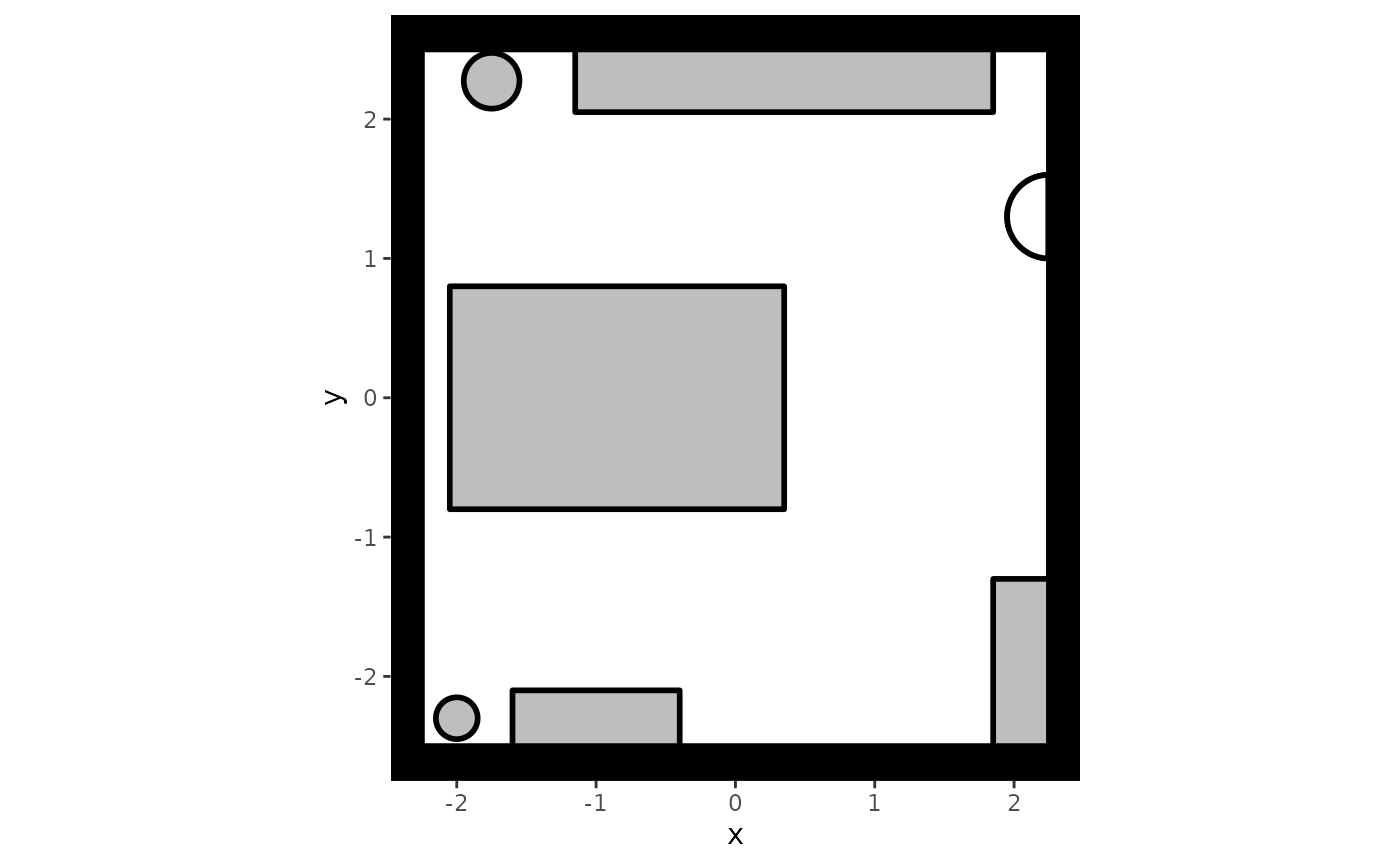

It is often useful to create your setting by going back and forth between adding an object and plotting the result, especially when the environment contains many different objects.

Interactability

By default, predped assumes that all objects in the environment can be interacted with. However, as this assumption may not apply to all situations, we also allow users to limit the interactability of the objects in their environment. This is done in two ways.

First, users can make a complete object non-interactable by setting the interactable argument of the constructors for rectangles, polygons, and circles to FALSE, such as in the following examples:

# Turn off interactability of the objects
my_rectangle <- rectangle(
  center = c(0, 0), 
  size = c(1, 1), 
  interactable = FALSE
)

my_polygon <- polygon(
  points = rbind(
    c(1, 1), 
    c(1, -1), 
    c(-1, -1), 
    c(-1, 1)
  ),
  interactable = FALSE
)

my_circle <- circle(
  center = c(0, 0), 
  radius = 1, 
  interactable = FALSE
)

Please note that if none of the objects in a given background are interactable, agents will enter the space and immediately leave again through one of the provided exits.

Another way in which interactability can be limited is through specifying the forbidden_edges argument in the same constructors. Essentially, this argument tells predped which regions of the objects cannot be interacted with. For polygons and rectangles, this amounts to providing the indices of the edges that cannot be interacted with, for example:

my_polygon <- polygon(
  points = rbind(
    c(1, 1), 
    c(1, -1), 
    c(-1, -1), 
    c(-1, 1)
  ), 
  forbidden = c(1, 3)
)

and defining $P_1 = (1, 1)$ , $P_2 = (1, -1)$ , $P_3 = (-1, -1)$ , and $P_4 = (-1, 1)$ , then the edges that cannot be interacted with are the lines $\overset{\leftrightarrow}{P_1 P_2}$ and $\overset{\leftrightarrow}{P_3 P_4}$ . This can be seen by executing the following code:

# Create the edges by extracting the coordinates that make up the polygon and 
# then combining them in fixed order
coords <- points(my_polygon)
edges <- cbind(coords, coords[c(2:nrow(coords), 1), ])

# Identify those edges that cannot contain a goal
idx <- forbidden(my_polygon)
edges[idx, ]
#>      [,1] [,2] [,3] [,4]
#> [1,]    1    1    1   -1
#> [2,]   -1   -1   -1    1

The same ideas apply to the rectangle, using the output of the points method to create the relevant edges.

For circles, there are no discrete edges that can be indexed like for polygons and rectangles. Within predped, we therefore use angles to specify the locations on the circle that cannot be interacted with, taking the shape of a matrix containing the starting and the ending angles of the interval in which no goal can be contained. Consider the following example, where we create a circle that cannot contain a goal in the region $[0, \pi]$ .

# Define a circle with forbidden angles ranging from 
# 0 to pi
my_circle <- circle(
  center = c(0, 0), 
  radius = 1, 
  forbidden = matrix(c(0, pi), nrow = 1)
)

Note that the angles should be specified in radians, not in degrees.

To simplify the specification of the forbidden argument, users can visualize the non-interactable locations when visualizing the environment. Redefining our office to include non-interactable locations:

# Adjust the office to contain forbidden edges
my_background <- background(
  shape = rectangle(
    center = c(0, 0), 
    size = c(4.5, 5)
  ), 

  objects = list(
    rectangle(
      center = c(-0.85, 0), 
      size = c(2.4, 1.6),
      forbidden = 1
    ), 
    rectangle(
      center = c(-1, -2.3), 
      size = c(1.2, 0.4), 
      forbidden = c(1, 3, 4)
    ), 
    rectangle(
      center = c(2.05, -1.9), 
      size = c(0.4, 1.2), 
      forbidden = 2:4
    ), 
    rectangle(
      center = c(0.35, 2.275), 
      size = c(3, 0.45), 
      forbidden = 1:3
    ),
    circle(
      center = c(-1.75, 2.275), 
      radius = 0.2, 
      forbidden = rbind(
        c(0, 5 * pi / 4),
        c(7 * pi / 4, 2 * pi)
      )
    ),
    circle(
      center = c(-2, -2.3), 
      radius = 0.15,
      forbidden = rbind(
        c(0, pi / 4),
        c(3 * pi / 4, 2 * pi)
      )
    )
  ), 

  entrance = c(2.25, 1.3)
)

We can then visualize these locations as through calling the plot method:

# Plot the background with forbidden locations
plot(
  my_background, 
  plot_forbidden = TRUE,
  forbidden.color = "red"
)

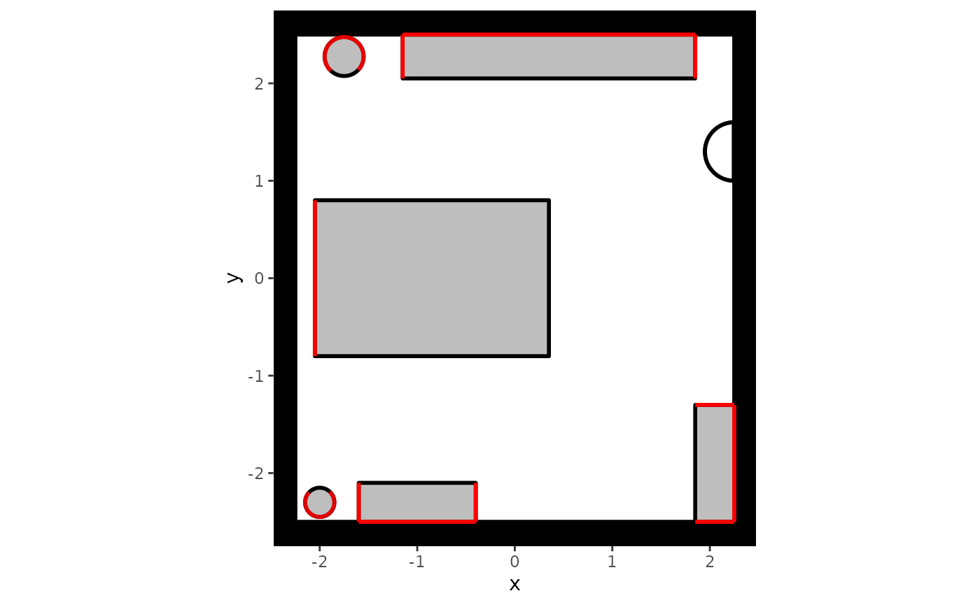
In this plot, non-interactable locations are visualized in red.

Note that interactability of an object will automatically be limited by where the objects are placed in the environment. More concretely, agents cannot interact with locations that they cannot reach, such as sides of an object that stand against another object or a wall. You do not need to specify this explicitly, though it may help during the setup of your simulation study.

Debugging

There are some known issues or limitations regarding the background class that users should be aware off when creating their own environments. These are included here:

Instances of the segment class cannot be included as an object in the objects argument, as they solely exist to restrict the directionality of the pedestrian flow within an environment.

Defining Agents

Once an environment has been defined, one should define the characteristics of the agents that are expected to walk around in this environment. The mapping of the setting with the agents is achieved through specifying an instance of the predped class. It has the following attributes:

setting: An instance of the background class defining the environment in which agents should walk around;
archetypes: A character vector containing the names of the types of agents you want to include;
weights: A numerical vector denoting the probability with which each agent type can be found within the environment;
parameters: A list containing all necessary parameter information for predped to be able to simulate distinct agents.

One can create an instance of the predped class through its constructor, for example by calling:

# Create instance of predped class with our office and the default 
# parameters
my_predped <- predped(setting = my_background)    
my_predped
#> Model object:
#> ID: model eqmfa 
#> Parameters taken from the BaselineEuropean, BigRushingDutch, DrunkAussie, CautiousOldEuropean, Rushed, Distracted, BaselineEuropean1, BigRushingDutch1, DrunkAussie1, CautiousOldEuropean1, Rushed1, Distracted1, Lost, SociallyAnxious, SocialBaselineEuropean, SocialBigRushingDutch, SocialDrunkAussie, SocialCautiousOldEuropean archetypes.

This specification connects the previously defined environment to the type of agents that should walk around in it. By default, all archetypes defined in the project’s can join the simulation with an equal probability. If you wish to limit the number of types of agents that can walk around in the simulation and/or wish to change these probabilities, one can specify the archetypes and weights arguments of the constructor. For example, specifying:

# Create instance of predped class with our office and two of the 
# default agent-types
my_predped <- predped(
  setting = my_background, 
  archetypes = c(
    "BaselineEuropean", 
    "DrunkAussie"
  ),
  weights = c(0.75, 0.25)
)
my_predped
#> Model object:
#> ID: model amrew 
#> Parameters taken from the BaselineEuropean, DrunkAussie archetypes.

states that you only want "BaselineEuropean"s and `“DrunkAussie”’s to walk around in the environment, where the former has a 75% probability of joining the environment while the latter only has a 25% probability of doing so.

Parameters

Given the importance of knowing which agent-types exist by default, and given the importance of personalization in specifying the agent characteristics (see Advanced Simulations), it is useful to explain the parameter structure used by predped.

To do so, we first load the default parameters of the package with the load_parameters function and inspect its type and structure:

params <- load_parameters()

typeof(params)
#> [1] "list"
names(params)
#> [1] "params_archetypes" "params_sigma"      "params_bounds"

As one can see, the variable params is a named list containing the slots "params_archetypes", "params_sigma", and "params_bounds". Each slot serves a different purpose in the specification of agents, as we detail below.

First, the "params_archetypes" slot contains a data.frame connecting the names of the agent types with the parameters that belong to this type. The data.frame contains the following columns:

colnames(params$params_archetypes)
#>  [1] "name"                  "color"                 "radius"               
#>  [4] "slowing_time"          "preferred_speed"       "randomness"           
#>  [7] "stop_utility"          "reroute"               "b_turning"            
#> [10] "a_turning"             "b_current_direction"   "a_current_direction"  
#> [13] "blr_current_direction" "b_goal_direction"      "a_goal_direction"     
#> [16] "b_blocked"             "a_blocked"             "b_interpersonal"      
#> [19] "a_interpersonal"       "d_interpersonal"       "b_preferred_speed"    
#> [22] "a_preferred_speed"     "b_leader"              "a_leader"             
#> [25] "d_leader"              "b_buddy"               "a_buddy"              
#> [28] "a_group_centroid"      "b_group_centroid"      "b_visual_field"       
#> [31] "central"               "non_central"           "acceleration"         
#> [34] "constant_speed"        "deceleration"

The column name contains the name of the agent type, color contains the color that is used to visualize the agent in simulation plots, and radius determines the size of the agent. After these initial three columns follow a bunch of parameters used by the utility functions on the operational level, namely:

randomness: Controls the randomness of the decisions of the agent;
stop_utility: Controls the utility of stopping instead of moving, forming a threshold that moving options need to surpass;
reroute: Controls the agent’s tendency to reroute when their route is blocked by other agents;
a_turning, b_turning: Controls the biomechanical limitations in the maintainence of your speed while turning;
preferred_speed, a_preferred_speed, b_preferred_speed: Parameters that control the utility of continuing to move at your preferred speed;
slowing_time: Controls the time needed for the agent to slow down when approaching a goal;
a_goal_direction, b_goal_direction: Controls the extent to which agents will head directly in the direction of their goals;
a_current_direction, b_current_direction: Controls the extent to which agents will continue to head in their current direction;
blr_current_direction: Controls a left-right side bias when overtaking or crossing other agents;
a_interpersonal_distance, b_interpersonal_distance, d_interpersonal_distance: Controls the extent to which agents leave room between them and other agents;
a_blocked_angle, b_blocked_angle: Controls the extent to which agents will anticipate and avoid directions that are blocked by other agents or objects at a distance;
a_leader, b_leader, d_leader: Controls the extent to which agents will follow a leader in crowded situations;
a_buddy, b_buddy: Controls the extent to which agents will walk besides others of the ingroup:
a_group_centroid, b_group_centroid: Controls the extent to which agents within a social group will tend to stick together;
b_visual_field: Controls the extent to which agents within a social group will try to keep each other in a field of vision.

The parameter names follow a particular convention, where for the typical utility function we use a is used for an exponent, b for a slope, and d for a difference between ingroup and outgroup members before the underscore _, and the name of the utility function after.

The values contained within this data.frame represent average values for the parameter for each agent type. For example, changing an agent type’s preferred_speed to a higher value means that this type of agent will tend to walk faster. Yet, one typically expects agents within a particular type to show quantitative differences from their prototype. This variation is handled by the "params_sigma" slot in the params variable.

The "params_sigma" slot contains a named list of matrices, each slot of which is named after the different agent types and the contents of which define the (co)variation of each of the parameters. For example, the variation matrix for the "BaselineEuropean" looks like follows::

head(params$params_sigma$BaselineEuropean)
#>                 radius slowing_time preferred_speed randomness stop_utility
#> radius            0.15          0.0            0.00        0.0         0.00
#> slowing_time      0.00          0.1            0.00        0.0         0.00
#> preferred_speed   0.00          0.0            0.05        0.0         0.00
#> randomness        0.00          0.0            0.00        0.1         0.00
#> stop_utility      0.00          0.0            0.00        0.0         0.01
#> reroute           0.00          0.0            0.00        0.0         0.00
#>                 reroute b_turning a_turning b_current_direction
#> radius              0.0         0         0                   0
#> slowing_time        0.0         0         0                   0
#> preferred_speed     0.0         0         0                   0
#> randomness          0.0         0         0                   0
#> stop_utility        0.0         0         0                   0
#> reroute             0.1         0         0                   0
#>                 a_current_direction blr_current_direction b_goal_direction
#> radius                            0                     0                0
#> slowing_time                      0                     0                0
#> preferred_speed                   0                     0                0
#> randomness                        0                     0                0
#> stop_utility                      0                     0                0
#> reroute                           0                     0                0
#>                 a_goal_direction b_blocked a_blocked b_interpersonal
#> radius                         0         0         0               0
#> slowing_time                   0         0         0               0
#> preferred_speed                0         0         0               0
#> randomness                     0         0         0               0
#> stop_utility                   0         0         0               0
#> reroute                        0         0         0               0
#>                 a_interpersonal d_interpersonal b_preferred_speed
#> radius                        0               0                 0
#> slowing_time                  0               0                 0
#> preferred_speed               0               0                 0
#> randomness                    0               0                 0
#> stop_utility                  0               0                 0
#> reroute                       0               0                 0
#>                 a_preferred_speed b_leader a_leader d_leader b_buddy a_buddy
#> radius                          0        0        0        0       0       0
#> slowing_time                    0        0        0        0       0       0
#> preferred_speed                 0        0        0        0       0       0
#> randomness                      0        0        0        0       0       0
#> stop_utility                    0        0        0        0       0       0
#> reroute                         0        0        0        0       0       0
#>                 a_group_centroid b_group_centroid b_visual_field central
#> radius                         0                0              0       0
#> slowing_time                   0                0              0       0
#> preferred_speed                0                0              0       0
#> randomness                     0                0              0       0
#> stop_utility                   0                0              0       0
#> reroute                        0                0              0       0
#>                 non_central acceleration constant_speed deceleration
#> radius                    0            0              0            0
#> slowing_time              0            0              0            0
#> preferred_speed           0            0              0            0
#> randomness                0            0              0            0
#> stop_utility              0            0              0            0
#> reroute                   0            0              0            0

Note that this matrix is not a covariance matrix. Instead, it contains the standard deviations of each parameter on its diagonal and the correlations between each parameter on its off-diagonal, thus containing the following structure:

$\begin{equation} \Gamma = \begin{bmatrix} \sigma_1 & \rho_{12} & \cdots & \rho_{1p} \\ \rho_{21} & \sigma_{2} & \cdots & \rho{2p} \\ \vdots & \vdots & \ddots & \vdots \\ \rho_{p1} & \rho_{p2} & \hdots & \sigma_p \\ \end{bmatrix} \end{equation}$

where $p$ is the number of parameters.

Computing the covariance matrix can be achieved through the following equation, defining $\Lambda$ as a diagonal matrix containing the standard deviations of the parameters and $R$ as the matrix containing the correlations on its off-diagonal and $1$ ’s on its diagonal, we can construct the covariance matrix $\Sigma$ as follows:

$\begin{equation} \begin{split} \Sigma &= \Lambda R \Lambda^T \\ &= \Lambda R \Lambda \end{split} \end{equation}$ where $T$ denotes the transpose.

We additionally note that the covariance matrix $\Sigma$ does not act on the raw (bounded) values of the parameters defined by the data.frame in "params_archetypes". Instead, it acts on a transformed unbounded version of these parameters, as explained below. The nature of this transformation falls outside of the scope of this vignette.

The final slot of the parameter list is "params_bounds", a matrix containing the bounds of each of the parameters. By default, these bounds are the following:

params$params_bounds
#>                        [,1]    [,2]
#> radius                2e-01 3.0e-01
#> slowing_time          5e-01 2.5e+00
#> preferred_speed       1e-02 2.5e+00
#> randomness            1e-04 5.0e+00
#> stop_utility          1e+01 1.0e+06
#> reroute               2e+00 3.0e+01
#> b_turning             0e+00 1.0e+00
#> a_turning             0e+00 3.0e+00
#> b_current_direction   0e+00 2.0e+01
#> a_current_direction   0e+00 3.0e+00
#> blr_current_direction 5e-02 2.0e+01
#> b_goal_direction      0e+00 2.0e+01
#> a_goal_direction      0e+00 3.0e+00
#> b_blocked             5e-02 2.0e+01
#> a_blocked             0e+00 3.0e+00
#> b_interpersonal       0e+00 2.0e+01
#> a_interpersonal       0e+00 3.0e+00
#> d_interpersonal       0e+00 1.0e+00
#> b_preferred_speed     0e+00 2.0e+01
#> a_preferred_speed     0e+00 3.0e+00
#> b_leader              0e+00 3.2e+02
#> a_leader              0e+00 3.0e+00
#> d_leader              0e+00 2.2e+02
#> b_buddy               0e+00 2.2e+02
#> a_buddy               0e+00 3.0e+00
#> a_group_centroid      0e+00 4.0e+00
#> b_group_centroid      0e+00 2.0e+01
#> b_visual_field        0e+00 1.1e+02
#> central               0e+00 1.0e+00
#> non_central           0e+00 1.0e+00
#> acceleration          0e+00 1.0e+00
#> constant_speed        0e+00 1.0e+00
#> deceleration          0e+00 1.0e+00

Lower and upper bounds for each of the parameters are contained in the first and second column respectively. Importantly, these bounds imply a fixed minimal and maximal value for each of the parameters, a feature that is preserved when generating random parameters for each agent.

Because the process of generating parameters may be a little obscure, we allow users to visualize the variation in the parameters across agents through the plot_distribution function, which typically will be used in the following way:

# Save all separate components in separate variables
means <- params$params_archetypes
covariances <- params$params_sigma
bounds <- params$params_bounds

# Select the parameters of the BaselineEuropean
means <- means[means$name == "BaselineEuropean", ]
covariances <- covariances$BaselineEuropean

# Create a plot 
set.seed(1) # Set for reproducability purposes
plot_distribution(
  1000,
  mean = means,
  Sigma = covariances,
  bounds = bounds
)

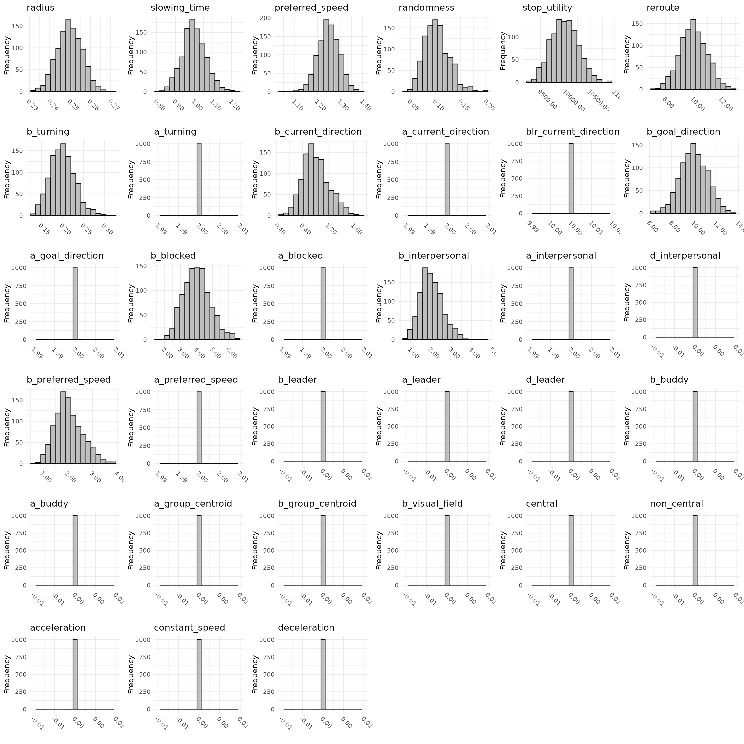
One sees a series of histograms displaying the randomly drawn values of the parameters across 1000 iterations, using the mean, covariance, and bounds specified in the variables `means`, `covariances`, and `bounds`.

For the default parameter settings, one can alternatively visualize the parameter distribution of a particular agent type as follows:

# Create a plot 
set.seed(1) # Set for reproducibility purposes
plot_distribution(
  1000,
  archetype = "BaselineEuropean"
)

which should output distributions similar to the previously plotted ones. Whichever way you use the function, it will output a set of histograms showing the variation in the values of each parameter with the current specifications of the three parameter slots. If you wish to play around with this, you can simply change the variables means, covariance, and bounds that were created earlier.

Performing the Simulation

With the hefty work done, we can finally go on to simulating pedestrian behavior as predicted by the M4MA. Having my_predped as the instance of the predped class that combines our environment with several agent characteristics, we can perform a simulation through calling the simulate function:

# Simulate behavior in our office for 100 iterations and maximally 3 agents
trace <- simulate(
  my_predped, 
  max_agents = 3, 
  iterations = 100
)
#> 
#> Precomputing edgesYour model: model amrew is being simulated

The variable trace is a list containing instances of the state class. Essentially, this class contains all information about the agents, environment, and other variables that are relevant for the simulation at each iteration. It has the following (relevant) slots:

iteration: The iteration number;
setting: The environment in which the agents are walking around;
agents: A list containing the agents that are currently present in the environment, each with their own characteristics, positions, orientations,…;
potential_agents: A list containing agents that are currently waiting at the entrance to enter the room;
variables: A named list containing variables that can be adjusted or used during the simulation (see Advanced Simulations);
iteration_variables: A data.frame containing information for the simulation at each iteration. Is slowly being phased out.

One can visualize both a single state of the simulation, or all states at once by calling the plot function:

# Plot a single state
plt <- plot(trace[[10]])
plt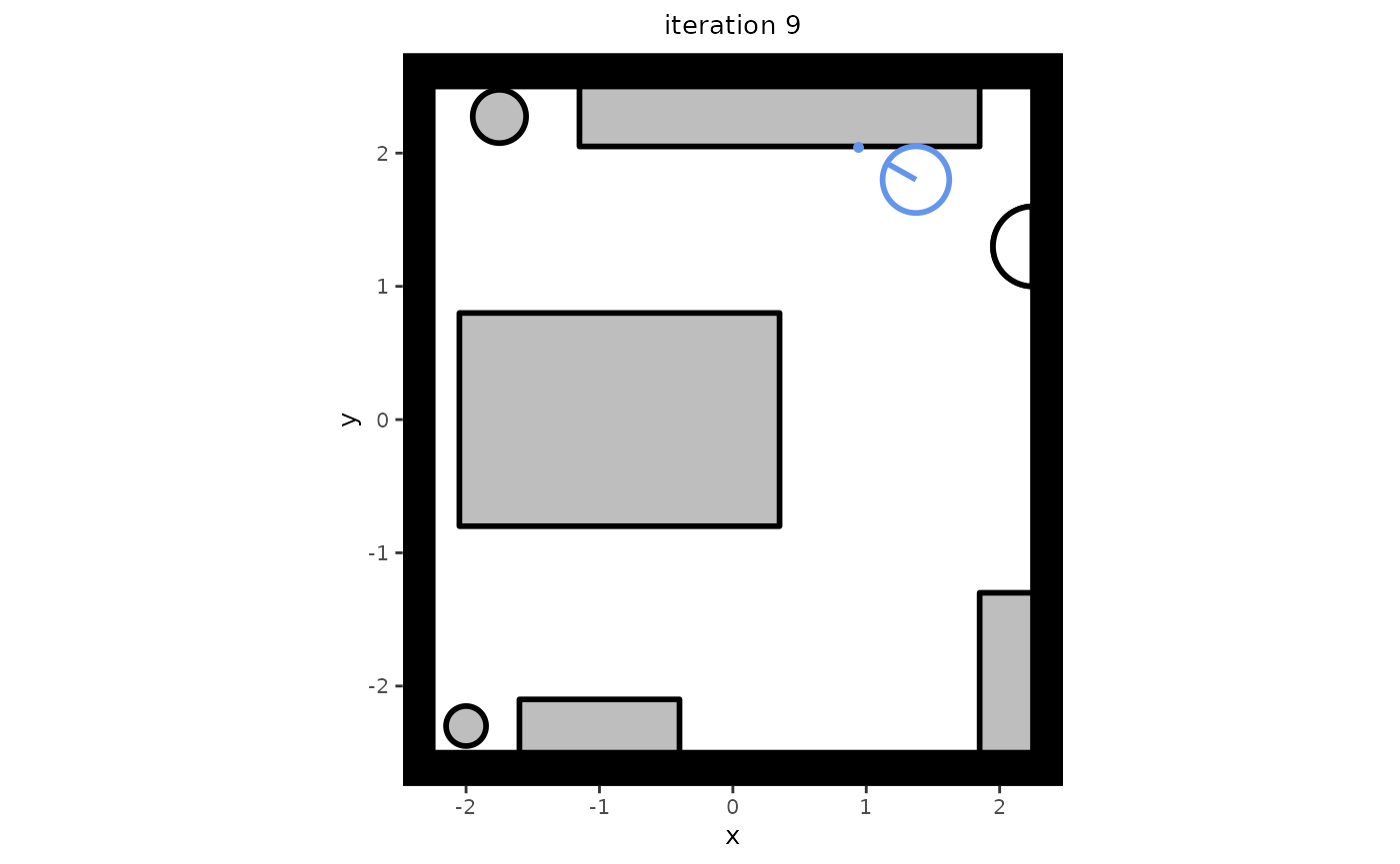

The plot shows the environment

# Plot the complete trace
plt <- plot(trace)

One can now skim through all plots to see how the agents behave, but this may turn out to be a tedious task. We therefore also recommend the creation of GIFs based on these plots. We recommend using the gifski package for this purpose:

# Create a GIF that is 5 times faster than real time (10 frames per second 
# instead of 2)
gifski::save_gif(
  lapply(plt, print), 
  file.path("my_gif.gif"),
  delay = 1/10
)

In our experience, this is the quickest way of producing a GIF in R, but we warn the user: When a trace is long, this may still take a while. If you are experimenting with simulation settings before running a full-length simulation study, we recommend setting the plot_live argument of simulate to TRUE instead. Note that plot_live is experimental and is known to not function equally well across different IDE’s.

Recap

In short, one can use the predped package to simulate data according to the M4MA by adhering to a particular workflow. Specifically, users need to specify (a) an environment, (b) the characteristics of the agents, and (c) the simulation characteristics. A minimal working example that combines all of these is shown the following bit of code:

# Load predped
library(predped)

# Create an environment: Simplified version of our office
my_background <- background(
  shape = rectangle(center = c(0, 0), size = c(4.5, 5)), 
  objects = list(
    # Desks
    rectangle(
      center = c(-0.85, 0), 
      size = c(2.4, 1.6),
      forbidden = 1
    ), 
    # Cabinets
    rectangle(
      center = c(-1, -2.3), 
      size = c(1.2, 0.4), 
      forbidden = c(1, 3, 4)
    ), 
    # Big bookcase
    rectangle(
      center = c(0.35, 2.275), 
      size = c(3, 0.45), 
      forbidden = c(1, 2, 3)
    )
  ), 
  entrance = c(2.25, 1.3)
)

# Link agent characteristics to the environment
my_predped <- predped(
  setting = my_background, 
  archetypes = c("BaselineEuropean", "DrunkAussie"),
  weights = c(0.5, 0.5)
)

# Simulate 120 iterations, or 1 minute
trace <- simulate(
  my_predped,
  max_agents = 3, 
  iterations = 120
)

# Plot the trace and save as a GIF
plt <- plot(trace)
gifski::save_gif(
  lapply(plt, print), 
  file.path("my_simulation.gif"),
  delay = 1/10
)