Estimation

One of the major advances of the Minds for Mobile Agents model (M4MA) is the ability to estimate its parameters on data. In this vignette, we will illustrate this through two examples, one starting from the trace output from the simulate function and the other starting from a data.frame containing measured movement data.

Note that for the estimation, predped only concerns itself with computing the utilities and associated probabilities of each expected movement decision. This means that we need to rely on external packages to perform the estimation procedure, using an optimization procedure to maximize the likelihood of the data under a set of parameters. Within this vignette, we use the nloptr package to perform this optimization procedure (Johnson, 2008). To install and use this package, one can execute the following two commands:

install.packages("nloptr")
library(nloptr)

For more information on the package and the NLopt library, we refer the interested reader to the dedicated documentation sites (nloptr: https://astamm.github.io/nloptr; NLopt: https://nlopt.readthedocs.io/en/latest).

Disclaimer

At the moment of writing, we are performing recovery studies to ensure the quality of the estimation of the M4MAs parameters. While likelihood profiles look good, we are not sure yet how much movement data is needed to ensure unbiased estimates with small standard errors. For now, we therefore do not guarantee accurate results when performing estimations on your own movement data.

Furthermore note that the computation of the likelihood has not been adequately optimzed yet. For large datasets, the estimation procedure may therefore be rather slow.

Starting from a Trace

Consider a trace that has been saved in the variable trace, containing a simulation in which people walk around in a minimal supermarket with some additional flow indicators to prevent blockages (see Advanced Simulations):

Then we need to perform the following steps to estimate the parameters of the M4MA to the data contained within this trace.

First, one will have to transform the trace to a data.frame, which can be achieved with the unpack_trace function:

data <- unpack_trace(trace)

The variable data contains a bunch of information in a variety of columns, namely:

colnames(data)
#>  [1] "iteration"   "time"        "id"          "x"           "y"          
#>  [6] "speed"       "orientation" "cell"        "group"       "status"     
#> [11] "goal_id"     "goal_x"      "goal_y"      "radius"      "agent_idx"  
#> [16] "check"       "ps_speed"    "ps_distance" "gd_angle"    "id_distance"
#> [21] "id_check"    "id_ingroup"  "ba_angle"    "ba_cones"    "fl_leaders" 
#> [26] "wb_buddies"  "gc_distance" "gc_radius"   "gc_nped"     "vf_angles"

Of these, some indicate some attributes of the agent at a particular time (e.g., position in x and y, speed and orientation in speed and orientation) but also the cell that they selected (cell) and variables that are relevant for computing the utility of that decision (e.g., check, ps_speed, gd_angle,…). The contents of the latter set of columns depend heavily on the requirements of the utility functions defined in the m4ma package and we refer the interested reader to its documentation for a full explanation (https://research-software-directory.org/software/m4ma).

Second, we need to delete datapoints that are not of interest for the estimation procedure. Given that the M4MAs parameters guide movement, we can only use those datapoints at which agents were moving around. Within a trace, the easiest way in which to spot whether this is the case is by filtering out any rows in which the utility variables are NA, indicating that they were not used during that iteration:

dim(data)
#> [1] 804  30

data <- data[!is.na(data$check), ]

dim(data)
#> [1] 419  30

Note that this step is not necessary for the code to run, but that a warning would be thrown in case NA are left in the data.

Finally, once the data has been filtered to contain only movement data, we can compute the likelihood of the data under a particular set of parameters. Calling this likelihood $L$, then one can compute the negative log-likelihood $-\log(L)$ with the mll function as follows:

# Define a set of parameters to be evaluated. For illustration purposes, we use
# the parameters of the DrunkAussie for this purpose. Note that we delete the 
# agent's type name and their color from the parameters. Furthermore note that 
# we need to transform the parameters to a numeric vector.
params <- load_parameters()$params_archetypes
params <- params[params$name == "DrunkAussie", -c(1, 2)] |>
  unlist() |>
  as.numeric()

# Compute the likelihood of the data under this parameter set
mll(
  data, 
  params,
  transform = FALSE,
  summed = TRUE
)
#>    grazd    ihvmf    mlchb    nxpju    womdz 
#> 196.1544 186.6085 142.5374 178.6028 142.5474

The output of this call to mll is a named vector displaying the summed negative log-likelihood of the data under the provided parameters.

In this piece of code, we specified the argument transform = FALSE to communicate that the provided parameters are on the bounded scale rather than the unbounded scale (see Parameters in the vignette on Simulations). When using an optimizer, it may be interesting to let the optimizer work on the unbounded (real) scale instead, in which case you can specify transform = TRUE. Additionally, we specified summed = TRUE to get the summed value for the negative log-likelihood across all datapoints of a particular agent. If you wish to see the values of the negative log-likelihood for each datapoint individually, you can set summed = FALSE.

The call to the mll function will serve as the basic building block of the estimation procedure, which we dive more into in the next section.

Optimization

Typically, we want to estimate a set of unknown parameters to the data that is available to us. To achieve this via the nloptr package, we need to first define an objective function, that is a function that outputs a value to be minimized by the optimizer through changing a vector of parameters that serve as an input to this function. In our case, the objective function will be a wrapper around the mll function, summing all of the negative log-likelihoods together into one single objective value:

objective_function <- function(parameters) {
  return(
    sum(
      mll(
        data, 
        parameters,
        transform = FALSE,
        summed = TRUE
      )
    )
  )
}

Note that this function only takes in a single argument parameters: The content of the data that is included in the call to mll is assumed to be a global variable. Furthermore note that for our purposes, we assume that the provided parameters fall on the bounded scale and therefore don’t need to be transformed.

Once the objective function is defined, we can call the nloptr function of the nloptr package to perform the estimation procedure. Using the dividing rectangles algorithm (Jones et al., 1993), for example, we get:

# Extract the bounds of the parameters
bounds <- load_parameters()$params_bounds

# Define the initial condition for the algorithm. Take the middle of the 
# interval defined by the bounds
x0 <- rowMeans(bounds)

# Perform the estimation procedure
fit <- nloptr(
  x0,
  objective_function, 
  lb = bounds[, 1],
  ub = bounds[, 2],
  opts = list(
    algorithm = "NLOPT_GN_DIRECT",
    maxeval = 1000,
    xtol_abs = 1e-4,
    ftol_abs = 1e-4
  )
)

# Print the resulting fit
fit
#> 
#> Call:
#> nloptr(x0 = x0, eval_f = objective_function, lb = bounds[, 1], 
#>     ub = bounds[, 2], opts = list(algorithm = "NLOPT_GN_DIRECT", 
#>         maxeval = 1000, xtol_abs = 1e-04, ftol_abs = 1e-04))
#> 
#> 
#> Minimization using NLopt version 2.10.0 
#> 
#> NLopt solver status: 5 ( NLOPT_MAXEVAL_REACHED: Optimization stopped because 
#> maxeval (above) was reached. )
#> 
#> Number of Iterations....: 1000 
#> Termination conditions:  maxeval: 1000   xtol_abs: 1e-04 ftol_abs: 1e-04 
#> Number of inequality constraints:  0 
#> Number of equality constraints:    0 
#> Current value of objective function:  739.726257900465 
#> Current value of controls: 0.25 1.5 2.085 4.166683 500005 16 0.5 1.5 10 1.5 3.375 10 1.5 10.025 1.5 10 1.5 
#> 0.5 10 1.5 160 1.5 110 110 1.5 2 10 55 0.5 0.5 0.5 0.5 0.5

Individual Parameters

Up to now, we have assumed that each of the participants has the same parameter set underlying their movement data. More realistically, though, individuals differ in their walking tendencies, requiring us to estimate different parameters for each individual within our data.

To achieve this, we have to provide a matrix of parameter values to the mll function with rows indicating the individuals and the columns the parameters of interest. In practice, we therefore need to change the objective function so that:

# Get the number of participants in the study
n <- length(unique(data$id))

# Define the objective function
objective_function <- function(parameters) {
  # Transform the parameters to the required format
  parameters <- matrix(
    parameters,
    nrow = n, 
    ncol = 33
  )

  # Compute the objective
  return(
    sum(
      mll(
        data, 
        parameters,
        transform = FALSE,
        summed = TRUE
      )
    )
  )
}

Then, it’s just a matter of changing the initial conditions x0 and the bounds lb and ub in the nloptr function so that it matches the objective function, in this case:

# Extract the bounds of the parameters
bounds <- load_parameters()$params_bounds |>
  rep(each = n) |>
  matrix(nrow = 33 * n, ncol = 2)

# Define the initial condition for the algorithm. Take the middle of the 
# interval defined by the bounds
x0 <- rowMeans(bounds)

# Perform the estimation procedure
fit <- nloptr(
  x0,
  objective_function, 
  lb = bounds[, 1],
  ub = bounds[, 2],
  opts = list(
    algorithm = "NLOPT_GN_DIRECT",
    maxeval = 1000,
    xtol_abs = 1e-4,
    ftol_abs = 1e-4
  )
)

# Print the resulting fit
fit
#> 
#> Call:
#> nloptr(x0 = x0, eval_f = objective_function, lb = bounds[, 1], 
#>     ub = bounds[, 2], opts = list(algorithm = "NLOPT_GN_DIRECT", 
#>         maxeval = 1000, xtol_abs = 1e-04, ftol_abs = 1e-04))
#> 
#> 
#> Minimization using NLopt version 2.10.0 
#> 
#> NLopt solver status: 5 ( NLOPT_MAXEVAL_REACHED: Optimization stopped because 
#> maxeval (above) was reached. )
#> 
#> Number of Iterations....: 1000 
#> Termination conditions:  maxeval: 1000   xtol_abs: 1e-04 ftol_abs: 1e-04 
#> Number of inequality constraints:  0 
#> Number of equality constraints:    0 
#> Current value of objective function:  3598.79453227266 
#> Current value of controls: 0.25 0.25 0.2833333 0.2833333 0.2833333 1.5 1.5 1.5 0.8333333 2.166667 1.255 
#> 0.425 1.255 0.425 2.085 2.50005 2.50005 2.50005 0.8334167 2.50005 500005 500005 
#> 500005 500005 500005 16 16 16 16 16 0.5 0.5 0.5 0.5 0.5 1.5 1.5 1.5 1.5 1.5 10 
#> 10 10 10 10 1.5 1.5 1.5 1.5 1.5 10.025 10.025 10.025 10.025 10.025 10 10 10 10 
#> 10 1.5 1.5 1.5 1.5 1.5 10.025 10.025 10.025 10.025 10.025 1.5 1.5 1.5 1.5 1.5 
#> 10 10 10 10 10 1.5 1.5 1.5 1.5 1.5 0.5 0.5 0.5 0.5 0.5 10 10 10 10 10 1.5 1.5 
#> 1.5 1.5 1.5 160 160 160 160 160 1.5 1.5 1.5 1.5 1.5 110 110 110 110 110 110 110 
#> 110 110 110 1.5 1.5 1.5 1.5 1.5 2 2 2 2 2 10 10 10 10 10 55 55 55 55 55 0.5 0.5 
#> 0.5 0.5 0.5 0.5 0.5 0.5 0.5 0.5 0.5 0.5 0.5 0.5 0.5 0.5 0.5 0.5 0.5 0.5 0.5 0.5 
#> 0.5 0.5 0.5

In this case, it may be useful to transform the parameters back to the matrix introduced in the objective function and provide it with matching column names denoting the parameters and row names denoting the participants themselves:

# Get the parameter names: By default the same order as the one in bounds
params <- load_parameters()$params_bounds |>
  rownames()

# Get the id names: The same order as the ones output by mll
ids <- mll(data, bounds[, 1], transform = FALSE) |>
  names()

# Transform the result to a matrix with the provided column and row names
fit$solution |>
  matrix(nrow = length(ids), ncol = length(params)) |>
  `rownames<-` (ids) |>
  `colnames<-` (params)
#>          radius slowing_time preferred_speed randomness stop_utility reroute
#> grazd 0.2500000    1.5000000           1.255  2.5000500       500005      16
#> ihvmf 0.2500000    1.5000000           0.425  2.5000500       500005      16
#> mlchb 0.2833333    1.5000000           1.255  2.5000500       500005      16
#> nxpju 0.2833333    0.8333333           0.425  0.8334167       500005      16
#> womdz 0.2833333    2.1666667           2.085  2.5000500       500005      16
#>       b_turning a_turning b_current_direction a_current_direction
#> grazd       0.5       1.5                  10                 1.5
#> ihvmf       0.5       1.5                  10                 1.5
#> mlchb       0.5       1.5                  10                 1.5
#> nxpju       0.5       1.5                  10                 1.5
#> womdz       0.5       1.5                  10                 1.5
#>       blr_current_direction b_goal_direction a_goal_direction b_blocked
#> grazd                10.025               10              1.5    10.025
#> ihvmf                10.025               10              1.5    10.025
#> mlchb                10.025               10              1.5    10.025
#> nxpju                10.025               10              1.5    10.025
#> womdz                10.025               10              1.5    10.025
#>       a_blocked b_interpersonal a_interpersonal d_interpersonal
#> grazd       1.5              10             1.5             0.5
#> ihvmf       1.5              10             1.5             0.5
#> mlchb       1.5              10             1.5             0.5
#> nxpju       1.5              10             1.5             0.5
#> womdz       1.5              10             1.5             0.5
#>       b_preferred_speed a_preferred_speed b_leader a_leader d_leader b_buddy
#> grazd                10               1.5      160      1.5      110     110
#> ihvmf                10               1.5      160      1.5      110     110
#> mlchb                10               1.5      160      1.5      110     110
#> nxpju                10               1.5      160      1.5      110     110
#> womdz                10               1.5      160      1.5      110     110
#>       a_buddy a_group_centroid b_group_centroid b_visual_field central
#> grazd     1.5                2               10             55     0.5
#> ihvmf     1.5                2               10             55     0.5
#> mlchb     1.5                2               10             55     0.5
#> nxpju     1.5                2               10             55     0.5
#> womdz     1.5                2               10             55     0.5
#>       non_central acceleration constant_speed deceleration
#> grazd         0.5          0.5            0.5          0.5
#> ihvmf         0.5          0.5            0.5          0.5
#> mlchb         0.5          0.5            0.5          0.5
#> nxpju         0.5          0.5            0.5          0.5
#> womdz         0.5          0.5            0.5          0.5

Unbounded Estimation

The algorithm that we used before requires us to impose bounds on the parameters. In some cases, however, it may be more useful to use an optimizer that operates on the real scale, rather than on a bounded one. In this case, we change the argument transform to TRUE and change the call to nloptr as follows:

# Change the objective function to operate on the real scale
objective_function <- function(parameters) {
  return(
    sum(
      mll(
        data, 
        parameters,
        transform = TRUE,
        summed = TRUE
      )
    )
  )
}

# Change the initial condition
x0 <- numeric(33)

# Perform the estimation procedure with an algorithm that does not require 
# bounds to be specified
fit <- nloptr(
  x0,
  objective_function, 
  opts = list(
    algorithm = "NLOPT_LN_SBPLX",
    maxeval = 1000,
    xtol_abs = 1e-4,
    ftol_abs = 1e-4
  )
)

# Print the resulting fit
fit
#> 
#> Call:
#> 
#> nloptr(x0 = x0, eval_f = objective_function, opts = list(algorithm = "NLOPT_LN_SBPLX", 
#>     maxeval = 1000, xtol_abs = 1e-04, ftol_abs = 1e-04))
#> 
#> 
#> Minimization using NLopt version 2.10.0 
#> 
#> NLopt solver status: 5 ( NLOPT_MAXEVAL_REACHED: Optimization stopped because 
#> maxeval (above) was reached. )
#> 
#> Number of Iterations....: 1000 
#> Termination conditions:  maxeval: 1000   xtol_abs: 1e-04 ftol_abs: 1e-04 
#> Number of inequality constraints:  0 
#> Number of equality constraints:    0 
#> Current value of objective function:  429.316084129412 
#> Current value of controls: -2.594467 -0.5634537 0.5070385 -0.2047041 0.6581698 0.2549867 0.2549867 
#> 0.06491596 -1.421626 -0.4919096 -0.0133553 10.21004 -0.3960335 -0.6823948 
#> -0.004831927 -0.3530833 -0.01361795 -11.13464 0.2360346 0.7072078 -2.224339 
#> 7.560695 0.2549867 0.2549867 0.2549867 0.2549867 0.2549867 0.2549867 0.2549867 
#> 0.2549867 0.2549867 0.2549867 -0.1656554

Importantly, the parameters now have been estimated to be on the real scale, yet the parameters of the M4MA need to be defined on the bounded scale. To transform the parameters to their proper values, we use the to_bounded function:

# Get the bounds of the parameters
bounds <- load_parameters()$params_bounds

# Extract the parameters and transform to a data.frame. Expected by the 
# to_bounded function
params <- fit$solution |>
  matrix(nrow = 1) |>
  as.data.frame() |>
  `colnames<-` (rownames(bounds))

# Use to_bounded to transform the parameters
transformed <- to_bounded(
  params, 
  bounds
)
transformed
#>           radius slowing_time preferred_speed randomness stop_utility  reroute
#> radius 0.2004737     1.073126        1.737901   2.094566     744788.1 18.81773
#>        b_turning a_turning b_current_direction a_current_direction
#> radius 0.6006333  1.577639            1.551349           0.9341749
#>        blr_current_direction b_goal_direction a_goal_direction b_blocked
#> radius               9.91871               20          1.03812  4.987519
#>        a_blocked b_interpersonal a_interpersonal d_interpersonal
#> radius  1.494217         7.24026        1.483702    4.254342e-29
#>        b_preferred_speed a_preferred_speed b_leader a_leader d_leader  b_buddy
#> radius          11.86594          2.280844   4.1801        3 132.1393 132.1393
#>        a_buddy a_group_centroid b_group_centroid b_visual_field   central
#> radius  1.8019         2.402533         12.01267       66.06967 0.6006333
#>        non_central acceleration constant_speed deceleration
#> radius   0.6006333    0.6006333      0.6006333    0.4342141

Starting from Data

Within predped, we also allow users to estimate the M4MA on their data directly. Consider the following dataset taken from a simplified train station, for example (see Advanced Simulations):

head(data)
#>       time passenger        x             y
#> 1 2.403958         1 4.692500  3.765789e-17
#> 2 2.932846         1 4.606273 -4.020823e-02
#> 3 3.413369         1 4.488606 -1.225997e-01
#> 4 4.063040         1 4.281833 -1.780042e-01
#> 5 4.453463         1 3.988913 -3.145950e-01
#> 6 4.992690         1 3.591787 -5.926661e-01

In this dataset, we measured the positions (x and y) of different passengers (passenger) at several time points (time). To go from this dataset to one that we can use for the estimation procedure, we need to take the following steps.

First, we need the dataset to conform to the standards of predped. This means that:

• The time variable needs to show discrete jumps conforming the time_step defined by the M4MA, it being $500$msec;
• A variable iteration needs to be added showing the iteration at which the positions were measured;
• The passenger variable needs to be renamed to the predped internal id.

Addressing the first change, this amounts to binning the data within a particular time window, aggregating the positions within that window through, for example, taking a mean, as we do in the next bit of code:

# Define the bins, assuming the time variable is specified in seconds
bins <- seq(
  min(data$time), 
  max(data$time) + 0.5, 
  by = 0.5
)

# Loop over the bins and aggregate the data within those bins. Take the average
# of the bin as the time indication. Do this for each person separately.
data <- lapply(
  unique(data$passenger),
  function(x) {
    data <- lapply(
      1:(length(bins) - 1),
      function(i) {
        # Select the relevant data, it being the data where the time lies within
        # a particular bin and the passenger is x
        idx <- data$time <= bins[i + 1] & data$time >= bins[i] & data$passenger == x
        selection <- data[idx, ]

        # Aggregate and return a single row of data
        if(nrow(selection) > 0) {
          return(
            data.frame(
              time = (bins[i] + bins[i + 1]) / 2,
              passenger = x,
              x = mean(selection$x),
              y = mean(selection$y)
            )
          )
        } else {
          return(NULL)
        }
      }
    )

    # Bind together and return
    return(do.call("rbind", data))
  }
)

# Bind all rows within the list of binned data together
data <- do.call("rbind", data)

# Order based on time
data <- data[order(data$time), ]

head(data)
#>         time passenger        x             y
#> 218 2.653958         1 4.692500  3.765789e-17
#> 219 3.153958         1 4.606273 -4.020823e-02
#> 220 3.653958         1 4.488606 -1.225997e-01
#> 221 4.153958         1 4.281833 -1.780042e-01
#> 222 4.653958         1 3.988913 -3.145950e-01
#> 223 5.153958         1 3.591787 -5.926661e-01

The iteration variable requires integer values denoting the bin in which the position was measured. To compute this variable, we can perform the following computation:

data$iteration <- (data$time - min(data$time)) / 0.5 + 1
head(data)
#>         time passenger        x             y iteration
#> 218 2.653958         1 4.692500  3.765789e-17         1
#> 219 3.153958         1 4.606273 -4.020823e-02         2
#> 220 3.653958         1 4.488606 -1.225997e-01         3
#> 221 4.153958         1 4.281833 -1.780042e-01         4
#> 222 4.653958         1 3.988913 -3.145950e-01         5
#> 223 5.153958         1 3.591787 -5.926661e-01         6

The column passenger can be renamed to id in the following way:

colnames(data)[2] <- "id"
head(data)
#>         time id        x             y iteration
#> 218 2.653958  1 4.692500  3.765789e-17         1
#> 219 3.153958  1 4.606273 -4.020823e-02         2
#> 220 3.653958  1 4.488606 -1.225997e-01         3
#> 221 4.153958  1 4.281833 -1.780042e-01         4
#> 222 4.653958  1 3.988913 -3.145950e-01         5
#> 223 5.153958  1 3.591787 -5.926661e-01         6

Now that the dataset conforms to predpeds standards, we have to compute the values of the input variables for the input functions. For this, we first need to translate the environment in which the data were collected to an instance of the background to the best of our abilities. In this case, we collected the data in a simplified train station that looks as follows:

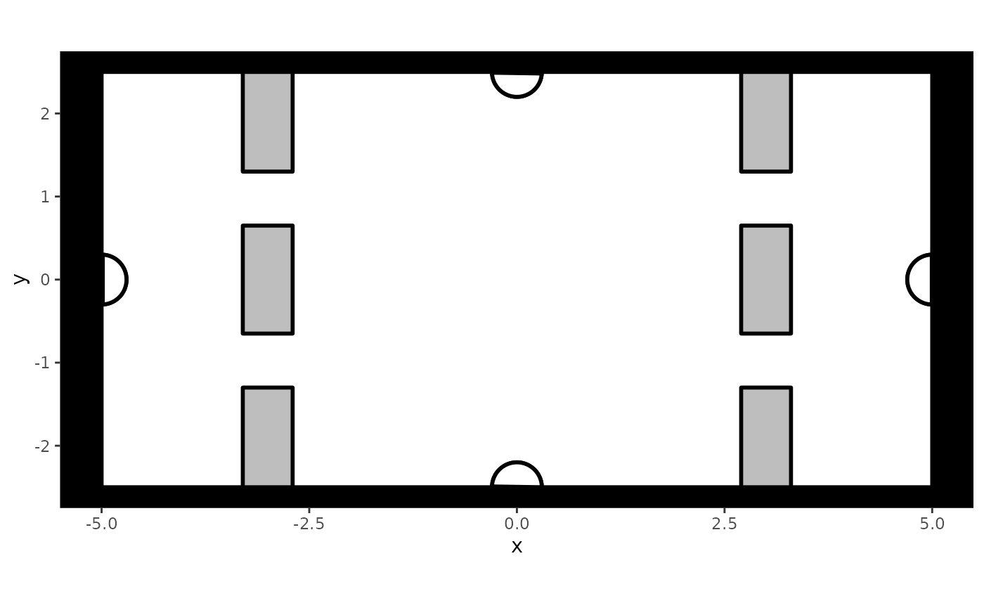
Note that when there are restrictions in flow, this is ideally included in the creation of this background (see Advanced Simulations).

Additionally, we need to include information on the goals that the people were trying to achieve within this environment, information that is necessary due to the M4MAs assumption that movement within space is guided by people’s goals. Specifically, we need to define the position of the goal as well as attach an identifier to this goal, each respectively contained in the goal_x, goal_y, and goal_id columns in the data. In this case, we know that each person was walking towards a particular exit of the space. Based on this information, we add the required columns as follows:

# Perform the mapping of a person with their goal position
mapping <- list(
  "exit 1" = c(1, 3, 12, 14, 21, 23, 28, 32, 33), 
  "exit 2" = c(2, 4, 5, 6, 9, 11, 16, 25),
  "exit 3" = c(7, 13, 18, 22, 24, 26, 30),
  "exit 4" = c(8, 10, 15, 17, 19, 20, 27, 29, 21)
)
coordinates <- list(
  "exit 1" = c(0, -2.5),
  "exit 2" = c(-5, 0),
  "exit 3" = c(0, 2.5),
  "exit 4" = c(5, 0)
)

# Add placeholders in the dataset for the columns to be filled later
data$goal_x <- 0
data$goal_y <- 0
data$goal_id <- " "

# Loop over the different mappings and fill the columns of interest
for(i in seq_along(mapping)) {
  # Define the rows to be filled based on the passengers moving to a particular
  # location
  idx <- data$id %in% mapping[[i]]

  # Fill the columns based on the exit's information
  exit <- names(mapping)[i]

  data$goal_x[idx] <- coordinates[[exit]][1]
  data$goal_y[idx] <- coordinates[[exit]][2]
  data$goal_id[idx] <- paste("moving to", exit)
}

head(data)
#>         time id        x             y iteration goal_x goal_y          goal_id
#> 218 2.653958  1 4.692500  3.765789e-17         1      0   -2.5 moving to exit 1
#> 219 3.153958  1 4.606273 -4.020823e-02         2      0   -2.5 moving to exit 1
#> 220 3.653958  1 4.488606 -1.225997e-01         3      0   -2.5 moving to exit 1
#> 221 4.153958  1 4.281833 -1.780042e-01         4      0   -2.5 moving to exit 1
#> 222 4.653958  1 3.988913 -3.145950e-01         5      0   -2.5 moving to exit 1
#> 223 5.153958  1 3.591787 -5.926661e-01         6      0   -2.5 moving to exit 1

Once the setting and the people’s goals have been defined, we can compute the input variables for the utility functions through the compute_utility_variables function as follows:

utility_data <- compute_utility_variables(
  data,
  train_station
)
colnames(utility_data)
#>  [1] "iteration"   "time"        "id"          "x"           "y"          
#>  [6] "speed"       "orientation" "cell"        "group"       "status"     
#> [11] "goal_id"     "goal_x"      "goal_y"      "radius"      "agent_idx"  
#> [16] "check"       "ps_speed"    "ps_distance" "gd_angle"    "id_distance"
#> [21] "id_check"    "id_ingroup"  "ba_angle"    "ba_cones"    "fl_leaders" 
#> [26] "wb_buddies"  "gc_distance" "gc_radius"   "gc_nped"     "vf_angles"

As shown, the result contains all of the same columns as the ones found in the transformed trace in the previous section. From here on, the steps to take in the estimation routine are thus the same and won’t be repeated.

References

Johnson, S. G. (2008). The NLopt nonlinear-optimization package. https://github.com/stevengj/nlopt

Jones, D. R., Perttunen, C. D., & Stuckmann, B. E. (1993). Lipschitzian optimization without the lipschitz constant. Journal of Optimization Theory and Applications, 79, 157.