Theoretical Framework

On this page, we provide the reader with a general introduction to the Minds for Mobile Agents (M4MA) pedestrian model. The model was developed as an alternative to physics-inspired pedestrian models that often assume pedestrian are all the same (e.g., Helbing & Molnár, 1995; Schadschneider et al., 2002). This is a reasonable assumption in crowds that are sufficiently dense to limit the expression of individual differences, but it limits the applicability of these models to only these high-density situations. The M4MA model aims to be more broadly applicable, allowing users to understand pedestrian behavior in both high- and low-density situations while accounting for the inherent heterogeneity that exists in pedestrians.

Building Blocks

The M4MA is based on the discrete-choice models of walking behaviour proposed by Antonini et al. (2006), Campanella et al. (2004), and Robin et al. (2009). These models fit within a broader utility-based framework proposed by Hoogendoorn & Bovy (2004) who proposed that pedestrians made decisions at three levels: (a) the strategic level that is concerned with the activities the pedestrians want to do within a particular environment, (b) the tactical level that is concerned with choosing a route to that location and adapting to changes in the environment, and (c) the operational level that is concderned with step-by-step decisions.

The M4MA makes a same distinction between the three interconnected levels of choice to understand pedestrian behavior. In the remainder of this text, we dive into the details of each level and how they are implemented in predped. If not done yet, it may be useful to take a look at the Getting Started page before engaging with this material.

Strategic Level

On the strategic level, the M4MA assumes that pedestrians plan a particular set of goals that they want to achieve within the environment. Before a pedestrian enters a room, they therefore already have a preplanned goal stack or collection of goals that they need to finish before they can leave the environment. For example, an agent can only leave a grocery store after finding all of the items they want to buy. Similarly, an agent who needs to catch a train can only do so after buying a ticket and finding the track at which the train leaves. The goal stack therefore plays an crucial role in guiding a pedestrian’s behavior: Without goals, there would be no movement.

According to the M4MA, goals contain two primary characteristics, namely a location (i.e., where to find the goal) and a timer (i.e., how long it takes to complete the goal). This allows agents to plan ahead on the order in which to achieve goals and defines how long they will interact with a particular goal, therefore controlling the length of periods of standstill as well as of movement. Note that this implies, though, that all agents have intimate knowledge about the space that they will walk into: Only then do they know exactly where to find their goals and how long they will take. For most purposes, however, this is a realistic assumption to take.

Within predped, the goal stack is contained within the agent itself, specifically under the slots current_goal and goal_stack. The former contains the goals that the agent currently wants to achieve while the latter contains goals that the agent needs to achieve later on. Each goal is furthermore coded as an instance of the goal class, containing the defining features id, position, and counter, representing an identifier, the location of the goal, and the number of iterations it takes to complete the goal.

Note that the strategic level’s role is retricted to what happens before the agent enters the room. When the agent has entered the room, the tactical and operational level take over. This is also reflected within the package: All functions related to the strategic level are called during the creation of an agent and are not used once the agent has been created. For more information on these functions, we refer the interested reader to the documentation of add_agent, add_group, and goal_stack.

Tactical Level

On the tactical level the M4MA places routing decisions, the manipulation of the goals within the goal stack, and other tactical decisions that influence the operational level. Regarding routing, the M4MA assumes that goals can be subdivided in two parts, namely activitiy goals which represent the end goal (e.g., getting the grocery item) and path points that represent locations that can be used to navigate the space between two points. Navigating the space from one’s current location to the end goal’s location therefore entails stringing together a series of path points within the space so as to end at the end goal’s location (see the Figure below). Importantly, this requires that an agent is able to see the next location that they move to (it being a path point or end goal). If this is not the case, the agent will choose one of several ways to resolve this issue, as we will detail below.

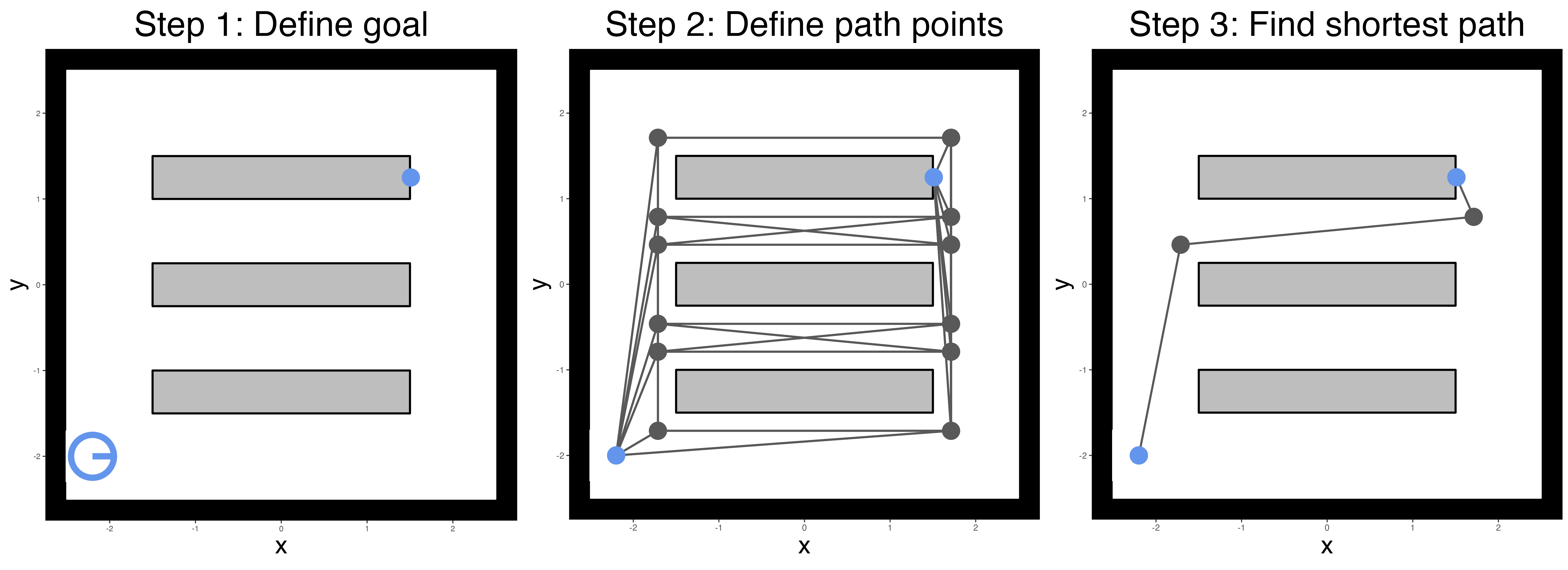
Within predped, path points are created and connected through the compute_edges function. To find the path from an agent’s location to their goal’s location, predped makes use of the find_path function, relying on a greedy algorithm implemented in the cppRouting package (Larmet, 2022), saving this path in the path slot in the relevant instance of the goal class.

Regarding goal manipulation, there are two ways in which agents can handle goals. First, they can reach a goal’s location and start interacting with the goal, waiting at the specified location for a determinate amount of time. In predped, this amounts to reducing the value of the counter slot by 1 at each iteration. Once the counter reaches 0, the goal is marked as completed and the first goal in the goal_stack is selected as the next goal to be achieved, first searching for the path towards that goal through the find_path function. Second, agents can decide that a particular goal is currently unreachable (e.g., when another agent is standing in the way), allowing them to switch to another goal. In this case, the current_goal is switched out for the first goal in the goal_stack, allowing them to return to the unachieved goal at a later time.

When an agent has reached the end of their goal stack (programmatically, when length(agent@goal_stack) == 0 and the current goal has been completed), then agents still need to leave the space. In predped, we assign a special type of goal for this purpose, namely one with the goal id "goal exit" and a position right before one of the exits of the space. This will prompt the agent to move towards an exit and, when close enough, set its status to "exit" to indicate that they are ready to leave the space (see the next paragraph).

Outside of routing and goal manipulation, the tactical level also encompasses several additional tactical decisions that influence the operational level. For one, agents have several ways of aleviating difficulties when they lose sight of their next path point or goal location, specifically by reorienting – turning in different directions and choosing one that provides a clear path – or rerouting – finding a new path to the goal location. Addditionally, agents can choose to wait for a specific amount of time, triggered only when either another agent is interacting with a goal close to theirs or when rerouting did not yield an alternative route. These types of decisions are capture through the status slot of the agent, in this case taking on the values "reorient", "reroute", and "wait" respectively. Other statuses of the agents are "move" (when an agent moves around), "completing goal" (when an agent is interacting with their goal), "plan" (when finding a path to their next goal), and "exit" (when the agent is ready to exit the space).

Another tactical decision is the agent’s tendency to slow down when they approach a goal location, preventing them from overshooting the goal (Robin et al., 2009). Within the M4MA, this adjustment is made at the tactical level, directly affecting the agent’s current speed so that they would arrive at the goal in particular time (by default 1sec or 2 iterations). Within predped, this is captured through the parameters slowing_time, which can be accessed through calling the load_parameters function.

Finally, tactics are also affected by group membership, which affects both the routing decisions of the group members as well as the value of some of the utility functions more directly. For example, agents in the same group typically don’t mind having a closer interpersonal distance to ingroup members rather than outgroup members or stick together more often. These tactical decision are captured within the utility functions at the operational level itself and will be elaborated on in that section.

Importantly, the tactical level can be used to accommodate situations where agents do not know goal locations and have to explore the area first to find their goals. For exmaple, in an earlier version of M4MA, agents could walk along the aisles in a supermarket before being able to see the items on their shopping list, adding their location to the goal stack as the next activity. More generally, the tactical level could be used to reconfigure other aspects of the model so that goals may influence the operational level (e.g., increasing agent’s preferred speed when their train is about to leave). Although not part of the default behavior in predped, we do provide ways for people to include their own set of tactical decisions of this level within simulations (see Advanced Simulations).

Operational Level

On the operational level, the M4MA describes how agents make step-by-step decisions while navigating the space. Step-by-step decisions are assumed to be taken once in a particular cycle, by default every 500msec. To guide this type of movement on the operational level, we first define all discrete step choices an agent has every cycle and then define the probability with which the agent chooses each discrete choice.

Discrete Step Choices

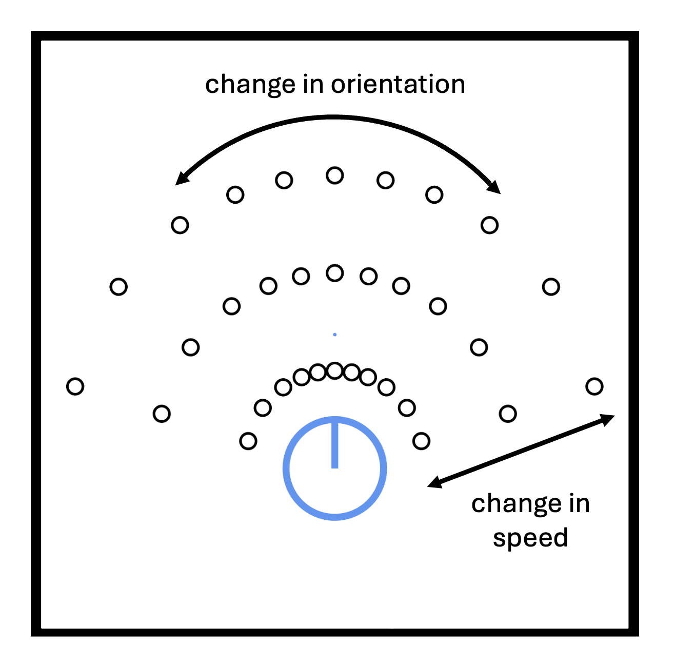
The M4MA states that on every cycle (by default 0.5sec) an agent chooses one of 34 discrete velocity options, 33 of which are composed by crossing 11 direction options or “cones” that describe turns relative to the current direction ($a \in \{-72.5^\circ, -50^\circ, -32.5^\circ, -20^\circ, -10^\circ, 0^\circ, 10^\circ, 20^\circ, 32.5^\circ, 50^\circ, 72.5^\circ\}$) and 3 speed options or “rings” that describe how speed changes relative the current speed ( multiplier $s \in \{0.5, 1, 1.5\}$; see the Figure below). The expansion of cones away from the center corresponds to direction control being more precise closer to the current direction.

Several things are of note here. First, as one may have noticed when examining the picture above, the M4MA includes a biomechanical slowing so that agents have difficulty maintaining or accelerating their speeds while turning. Within predped, this slowing factor is taken into account when computing these discrete choices in predpeds compute_centers and can be summarized mathematically as:

$$\begin{equation} \begin{split} \rho_i &= 1 - \beta_{turn} \text{sin}(\frac{|a_i|}{2})^{\alpha_{turn}} \\ s_i^* &= \rho_i s_i \end{split} \end{equation}$$ where $i \in \{1, 2, \cdots, 33\}$ represents the discrete choice of interest, $a_i$ is the turning angle for this choice, $s_i$ is the speed for this choice if the agent were not turning, $s_i^*$ represents the biomechanically corrected speed, and $\beta_{turn}$ and $\alpha_{turn}$ are the parameters that guide this biomechanical slowing. Within predped, we allow each agent to have a different rate of slowing as capture through their parameters b_turning and a_turning (see params_from_csv).

Additionally, under the hood we are required to index the rings and cones in a particular reproducible way. In predped, rings are numbered $r \in \{1, 2, 3\}$, with $r = 1$ corresponding to acceleration, $r = 2$ to maintaining speed, and $r = 3$ to decelerating. Cones are numbered $k \in \{1, \hdots, 11\}$ from left to right from the agent’s perspective. The set of locations corresponding to each option is described as a “cell” and the set of cells defines the agent’s spatial “field of operations” for the current cycle. Hence, each of these $i = \{1, \hdots, 33\}$ choices corresponds to moving to a new location and, typically, a change in direction and/or speed. The index for each of the cells is found by multplying the ring identifier with the cone identifier, so that cells are numbered $1, \hdots, 11$ from left to right in the acceleration ring, $12, \hdots, 22$ in the constant speed cone, and $23, \hdots, 33$ in the deceleration cone.

The 34th Option

In scenarios modeled by Antonini et al. (2006) and Robin et al. (2009), pedestrians were assumed to be always in motion. In contrast, the M4MA allows agents to stop for one of three reasons: (a) no cell is available (e.g., all cells are blocked by objects or other pedestrians in a crowded scenario), (b) one or more cells are available but none have an acceptably high utility (see later on), and (c) agents are performing an activity (e.g., buying a ticket). Hence, we added a 34$^{th}$ option that allows agents to stop, corresponding to the current location and direction being maintained while reducing their speed to zero. When movement subsequently recommences speed is set to a low value controlled through the standing_start argument of simulate.

Probability of Moving to a Cell

Once an agent has identified the positions that they can move to on the current cycle, they still need to make a decision between these different options. According to the M4MA, the probability that an agent will choose a specific cell $i \in \{1, ... 33\}$ is determined by that cell’s utility $u_i \in (-\infty, 0]$, denoting how useful it is for the agent to move to cell $i$. The larger the value of $u_i$, the greater the usefulness.

Using the utility $u_i$ of a particular cell, one can derive the probability of moving to that cell as:

$$\begin{equation} p_i = \frac{e^{\tau^{-1} u_i}}{Z}, \end{equation}$$

where $Z$ is a normalizing constant that ensures all probabilities add to 1 and $\tau$ is a randomness parameter which controls to which extent the agent always chooses the cell with the highest utility, where small values of $\tau$ make the agent’s decision process essentially deterministic (see the randomness parameter in params_from_csv). Using these probabilities, agent’s randomly select one of the options according to a multinomial distribution and, once selected, change their position to the chosen cell.

A two-stage procedure is used to determine each of the 33 cells’ utility. In the first stage, we set the utility of a particular cell to $-\infty$ when it is not accessible. This is the case when a cell is currently occupied or movement to the cell is obstructed by other objects and when moving to that location would require the agent’s body intersecting with other objects in the space. By setting the utility to $-\infty$ in these cases, we prevent the agent from being able to choose this cell so that its probability $p_i = 0$ at the current cycle. In predped, this check is taken care of by the moving_options function.

In the second stage, the utility of all available cells is computed as the weighted sum of M4MAs component utilities defined, each of which quantifies a preference regarding different aspects of the pedestrian’s behavior. For sake of simplicity, we set the maximum value for a particular component utility to $0$ so that utilities that become more negative indicate a decrease in their preference.

With these two steps in mind, we can define the utility of cell $i = \{1, \hdots, 33\}$ for agent $j$ as:

$$\begin{equation} u_{ij} = \begin{cases} \displaystyle\sum_{f \in F} f(S_j, \bm{x}_i | \bm{\theta}_f), & \quad{\text{if cell $i$ is available}} \\ -\infty, & \quad{\text{if cell $i$ is unavailable}} \end{cases}, \end{equation}$$ where $F$ indicates the set of component utility functions $f$, each of which takes in a matrix of agent states $S_j$, the position $\bm{x}_i$ of the cell $i$, and a set of parameters $\bm{\theta}_f$ specific to the utility function. Most utility function make use of a similar structure with an exponent parameter $\alpha_f$ and a weight parameter $\beta_f$. For some utlity functions, there is an additional weight parameter $\delta_f$ that is added to $\beta_f$, altering the utility of a particular cell based on an agent’s group membership.

Within predped, the parameter designations are reflected in the use of a notational convention, using a_<component> for $\alpha_f$, b_<component> for $\beta_f$, and d_<component> for $\delta_f$ (see params_from_csv). The agent states $S_j$ are furthermore included in the package as a combination of the current state (an instance of the state class) and several highlighted specifications of the agents within that space such as identifiers and predictions (the output of create_agent_specifications, allowing mapping to the utility functions contained in the m4ma package).

Up to now, we have only defined the utility of moving to one of the 33 new locations, but not about the utility of standing still. For this, the M4MA sets the utility of the agent’s $34^{th}$ cell to a fixed value $\upsilon_j$, ensuring agent’s will only stop when no other good options are available (i.e., when all utilities $u_{ij} < \upsilon_j$ in the deterministic case). The value of $\upsilon_j$ is contained in the parameter list of the agent as stop_utility (see again params_from_csv).

In the remainder of this section, we will highlight the different component utility functions that the M4MA uses to guide agent’s decisions on the operational level.

Component Utility Functions

The M4MA’s existing component utility functions can be divided along several different dimensions, namely (a) individual vs. social, (b) attractive vs. repulsive, and (c) predictive vs. concurrent. The individual-social dimension captures whether a utility function accounts for the agent’s own characteristics (individual) or those of the other agent’s in the space as well (social). The attractive-repulsive dimension furthermore specifies whether the utility function acts through attraction (attractive) or repulsion (repulsive) from a central point or region. The predictive-concurrent dimension finally specifies whether they make use of concurrent information (concurrent) or of predictions that the agent made (predictive). Predictions are always based on the other agents’ current speed and direction, allowing the agent to anticipate their locations on the next time step by assuming that they continue moving in the same direction and at the same speed.

The categorization of each utility functions with regard to these dimensions are displayed in the following Table.

Utility function	Abbreviation	Individual-Social	Attractive-Repulsive	Predictive-Concurrent
current direction	CD	individual	attractive	concurrent
goal direction	GD	individual	attractive	concurrent
preferred speed	PS	individual	attractive	concurrent
interpersonal distance	ID	social	repulsive	predictive
blocked angle	BA	social	repulsive	predictive
follow-the-leader	FL	social	attractive	predictive
walk-beside	WB	social	attractive	predictive
group centroid	GC	social	attractive	predictive
visual field	VF	social	attractive	predictive

In what follows, we give a detailed overview of the utility functions themselves. Note that all parameters that we discuss are assumed to be positively valued. Furthermore note that, for simplicities sake, we won’t index the different utility functions $f$ and parameters $\alpha$, $\beta$,… with their respective abbreviation for the utility function (e.g., CD for current direction), ensuring clean equations for each utility function.

Current Direction

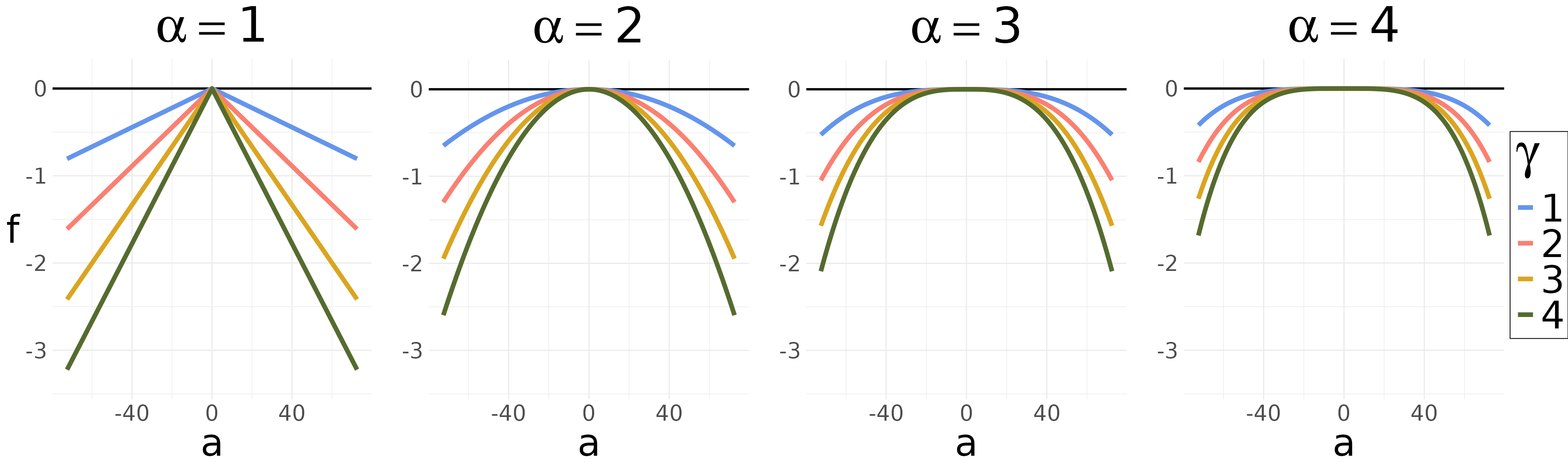
The current direction utility function creates a tendency for pedestrians to continue heading in their current direction. For each cell $i$ in the same cone $k$, this utility function returns the same value, being $0$ for the central cone ($k_i = 6$) and increasingly negative for cones on either side. Defining $a_{k_i}$ as the angle in degrees of the cone $k$ in which cell $i$ is contained, then the utility function is computed as:

$$\begin{equation} f_i = - \gamma \left|\frac{a_{k_i}}{90}\right|^{\alpha} . \end{equation}$$ Note that in this equation, the cone angles are normalized by the constant $90$ and the absolute value is taken, so that the resulting quantity is on the unit interval. The parameters $\alpha$ and the function $\gamma$ define the exponent and weight that determine the value of this utility function in the way displayed in the following figure:

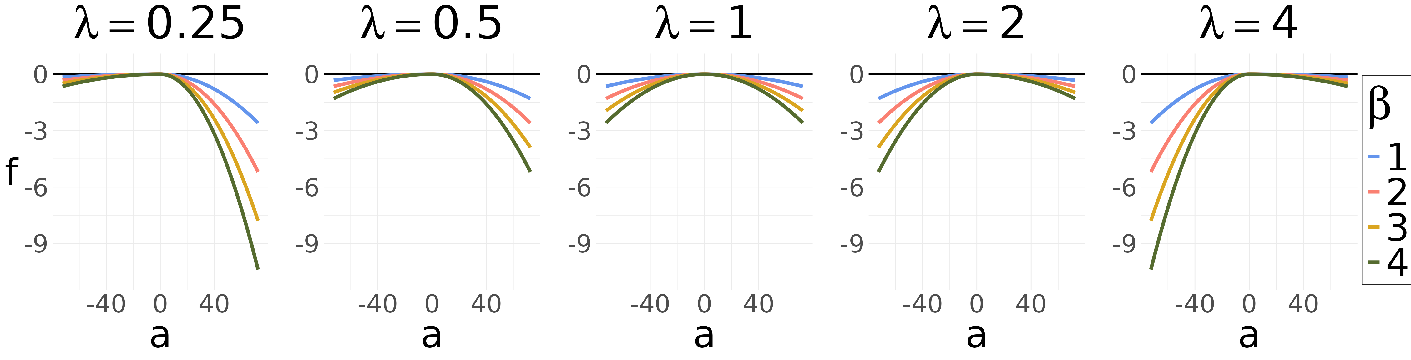
The parameter $\gamma$ in the utility function is defined in terms of the cone in which the cell $i$ is contained, the weight parameter $\beta$, and a side-bias parameter $\lambda$. If $\lambda = 1$ there is no side bias, if $\lambda < 1$ there is a bias to the left, and if $\lambda > 1$ there is a bias to the right:

$$\begin{equation*} \gamma = \begin{cases} \beta, & \quad{k_i = 6} \\ \beta \lambda, & \quad{k_i > 6} \\ \beta \lambda^{-1}, & \quad{k_i < 6} \end{cases} \end{equation*}$$

The effect of the parameter $\lambda$ on the utility is shown in the following figure.

Within predped, the parameters $\alpha$, $\beta$, and $\lambda$ are known as a_current_direction, b_current_direction, and blr_current_direction.

For identifiability purposes, we set b_current_direction = 1 for all archetypes uses in predped, weighing the influence of the other utility functions relative to this one.

Preferred Speed

The preferred speed utility function creates a tendency for pedestrians to keep to a particular speed. Consequently, it’s output is the same for all cells $i$ contained in a same ring $r_i$. Denoting the preferred speed as $\varsigma$, the current speed as $s$, and $s_{r_i}$ as the adjusted speed once the multiplier of the ring has been taken in to account (0.5 for deceleration, 1 for maintenance, and 1.5 for acceleration), then the preferred speed utility function is defined as:

$$\begin{equation} f_i = -\beta \left| s_{r_i} - \varsigma^* \right|^{\alpha}, \end{equation}$$ taking on the same shape as for the unbiased current direction utility function above. The preferred speed utility function thus attains an optimal utility of $0$ whenever the speed of a particular ring corresponds to the agent’s preferred speed. Note, however, that this equation does not make use of the raw preferred speed $\varsigma$, but rather of a value $\varsigma^*$ derived thereof. The value of $\varsigma^*$ depends on the distance $d$ between an agent and their goal, so that

$$\begin{equation} \varsigma^* = \text{min}( \varsigma, \tau \frac{\varsigma}{d} ) , \end{equation}$$ where $\tau$ is a time-based slowing parameter, ensuring that an agent approaches a goal more slowly in order to not overshoot its location.

In predped, the parameters $\varsigma$, $\tau$, $\beta$, and $\alpha$ are called preferred_speed, slowing_time, b_preferred_speed, and a_preferred_speed respectively.

Goal Direction

The goal direction utility function creates a tendency for pedestrians to head towards their goals. Like for the current direction utility function, its value is the same for all cells contained within a same cone. Let $g$ be the angle between the current direction and the goal, and denote $a_{k_i}$ as the angle of the cone in which cell $i$ is contained (in degrees). Then we normalize the absolute deviation by 90 degrees and define the utility function as:

$$\begin{equation} f_i = - \beta \left| \frac{a_{k_i} - g}{90} \right|^{\alpha} . \end{equation}$$

This utility functiona gain resembles the others already discussed, this time attaining a maximal value of $0$ when the goal direction aligns perfectly with the cone.

Interpersonal Distance

The interpersonal distance utility function creates a tendency to avoid other pedestrians, with its effects differing depending on whether the other pedestrians belong to the in- or outgroup. Let $d_{ij}$ be the shortest distance between the agent when standing in cell $i$ and another visible agent $j$ standing at its predicted position, then this utility function takes the average of a power function of all distances $d_{ij}$ across the set of visible agents $A_i$ at that cell $i$:

$$\begin{equation} f_i = -\frac{1}{N_i} \sum_{j \in A_i} \gamma d_{ij}^{-\alpha} , \end{equation}$$ where $N_i$ represent the number of visible agents in the list of agents $A_i$ visible from cell $i$. This equation defines a hyperbolic function for the distance to each individual agent, as visualized in the next Figure. Note that this utility function becomes $-\infty$ whenever the interpersonal distance $d_{ij}$ is $0$, ensuring that the agent does not choose a cell that would result in a collision.

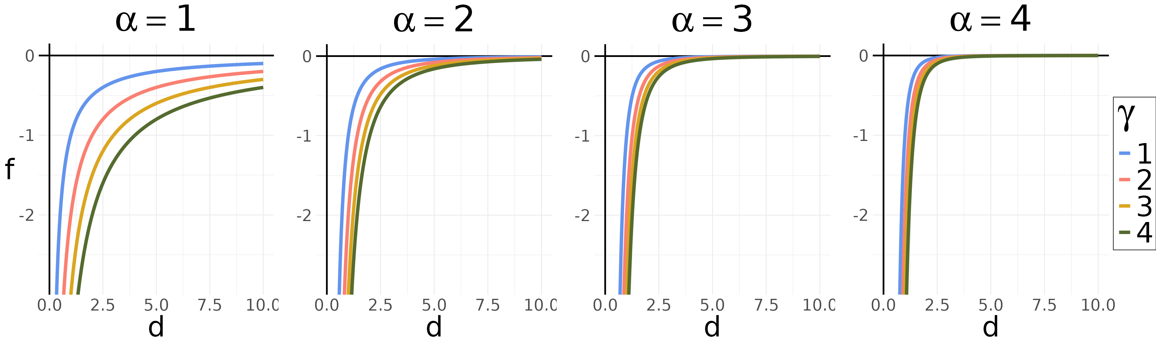
The interpersonal distance utility function critically depends on the parameter $\gamma$, which itself is a function of the weight parameter $\beta$ and the group membership of the other agent, so that:

$$\begin{equation} \gamma = \begin{cases} \beta, & \quad{\text{if agent $j$ is a member of the ingroup}} \\ \beta + \delta, & \quad{\text{if agent $j$ is not a member of the ingroup}} \end{cases} . \end{equation}$$ As demonstrated by Figure~, adding $\delta$ to $\beta$ decreases the utility of a cell, thus creating a tendency to avoid getting too close to out-group members.

In predped, the parameters $\alpha$, $\beta$, and $\delta$ for the interpersonal distance utility function are known as a_interpersonal, b_interpersonal, and d_interpersonal respectively.

Blocked Angle

The blocked angle utility function introduces the tendency to move in directions that afford a clear path, which can become particularly important in crowded situation. Its intent is to approximate an ability to avoid directions that are blocked by other agents before being forced to take a tactical decision (e.g., rerouting). Note that the blockage may lie both inside or outside the field of operations, increasing an agents’ ability to avoid collisions even if they are not likely to occur for several steps.

Blocking is assessed by computing the profile for the closest visible agent falling within each cone at any distance (see the Figure below). A profile is created by first connecting a line between agents then drawing a profile line perpendicular to the connecting line at the center of the other agent. The profile then is the line segment spanning the other agent’s diameter. A cone is considered “blocked” if an agent profile spans the edges of the cone (i.e., if there is no room within the cone to move past the blocking agent).

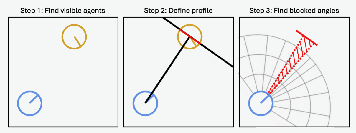
Any cell $i$ in a cone $k_i$ that is not blocked is given the maximal utility of $0$. For each cell in the other cones, a distance $d_i$ from the cell to the blocking agent is derived and the following utility function is computed:

$$\begin{equation} f_i = \begin{cases} 0, & \quad{\text{if cell $i$ not in a blocked cone}} \\ -\infty & \quad{\text{if blocking agent $j$ stands between the agent and cell $i$}} \\ -\beta d_{i}^{-\alpha}, & \quad{\text{if cell $i$ lies in a blocked cone}} \end{cases} . \end{equation}$$

This function takes on the same shape as for the interpersonal distance utility function.

In predped, the parameters alpha and \beta are stored as a_blocked and b_blocked.

Follow the Leader

The follow-the-leader utility function attracts a pedestrian towards currently occupied cells containing a potential “leader”, a close and visible agent who is heading in the general direction of the agent’s current goal. Importantly, this utility function assumes that the leader will move to a new position at the next time step, leaving their current cell available for occupation by the agent.

Computing this utility function requires several steps. First, we identify potential leaders for each cell $i$ (if any), selecting those agents who currently occupy cells within the agent’s field of operations. If multiple agents are selected for each cell, preference is given to those who belong to the agent’s ingroup and whose current direction is closest to the agent’s own goal direction. Selected agents are then designated as cell $i$’s leader.

For cells with a leader, we define the distance $d_{i, t + 1}$ from the leader’s predicted position on the next step $t + 1$ to the cell $i$ and the angular difference $a_{i}$ between the direction of the agent’s goal and cell’s leader (in degrees), allowing us to compute the follow-the-leader utility as follows:

$$\begin{equation} f_i = \begin{cases} 0, & \quad{\text{if cell $i$ does not have a leader}} \\ -\gamma \left| \frac{a_i}{90} \right| d_{i, t + 1}^{\alpha}, & \quad{\text{if cell $i$ has a leader}} \end{cases} . \end{equation}$$

As previously, we normalize the $a_i$ to fall on the unit interval. The shape of the utility function is shown in the next Figure. Note that in the case where the angular disparity is $0$, the utility is at its maximum value, meaning that leader’s who are heading in the same direction as the agent’s current goal are strongly preferred.

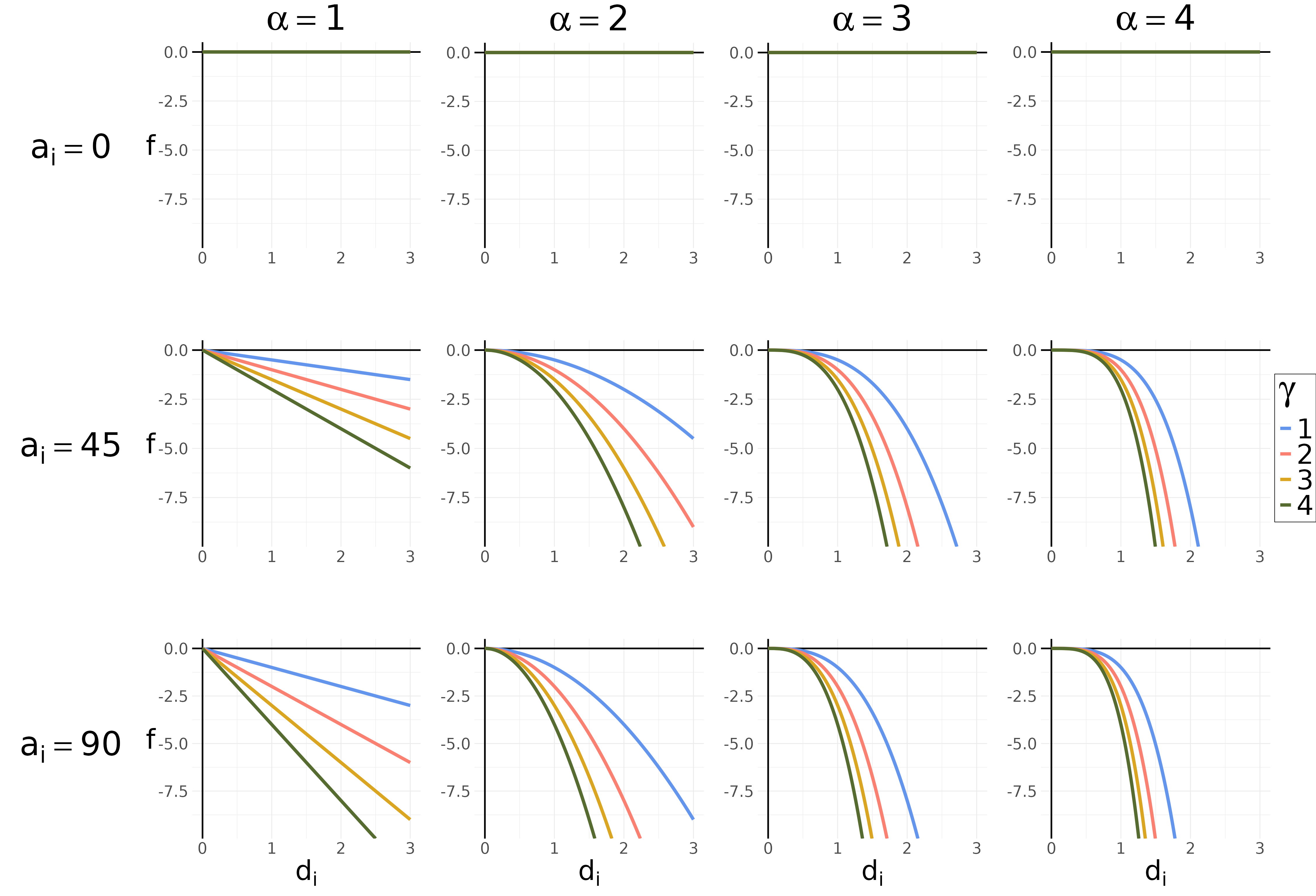
In the above equation, the parameter $\gamma$ changes based on the group membership of the leader, so that:

$$\begin{equation} \gamma = \begin{cases} \beta, & \quad{\text{if cell $i$'s leader is a member of the ingroup}} \\ \beta + \delta, & \quad{\text{if cell $i$'s leader is not a member of the ingroup}} \end{cases} . \end{equation}$$ Adding $\delta$ to $\beta$ will decrease the utility of using this agent as a leader, letting agents tend to use ingroup members as leaders.

In predped, the parameters $\alpha$, $\beta$, and $\delta$ controlling the follow the leader utility function are called a_leader, b_leader, and d_leader respectively.

Walk Beside

The walk beside utility function attracts agents towards cells that are located beside a “buddy”, a member of the ingroup. The aim of this utility is to approximate the tendency to walk beside group members in order to converse with them (cf. the other group utility function). Like for the follow the leader utility function, this utility function requires a few steps in its computation.

In a first step, potential buddies are identified through finding agents that belong to the ingroup and are reachable for the agent. Importantly, potential buddies do not need to be in the agent’s field of view, as it is assumed that pedestrians are usually aware of the locations of ingroup members even if they are cannot presently see them. This implies that the utility can slow down the agent when a potential buddy is reachable and behind them.

For each buddy $j$, we define their corresponding buddy cell as being the cell that lies (a) in the cone most parallel to the buddy’s current direction and (b) closest to the predicted position of the buddy on the next time step. We define the distance $d_{ij}$ each cell $i$ to the buddy cell $j$ and the angular difference $a_j$ between the current direction of the agent and the buddy and use these to compute the utility function as:

$$\begin{equation} f_i = -\sum_{j \in B} \beta \left| \frac{a_j}{90} \right| d_{ij}^{\alpha}, \end{equation}$$ where $B$ is the set of all buddies. Note that this utility function has the same shape as the follow the leader utility function, meaning one can refer to the previous figure for a visualization.

In predped, the parameters $\alpha$ and $\beta$ for the walk beside utility function are called a_buddy and b_buddy respectively.

Group Centroid

The group centroid utility function attracts agents towards the predicted position of their social group as a whole. The central assumption here is that different group members want to walk together as a group, rather than as separate individuals. This therefore represents a more extreme case than the walk beside utility function in which agents only temporarily join forces with ingroup members.

Define the group centroid as the mean predicted location $\bar{\bm{x}}$ across all group members and define the distance $d_i$ between a cell $i$ and the group centroid, then the group centroid utility function can be computed as:

$$\begin{equation} f_i = \begin{cases} 0, & \quad{\text{if $d_i <= \Delta$}} \\ -\beta | d_i - \Delta |^{\alpha}, & \quad{\text{if $d_i > \Delta$}} \end{cases} \end{equation}$$ where $\Delta$ is a comfortable distance around the group centroid that agents can maintain and for which the utility is optimal. Defining $\Delta$ makes sure that agents will remain close to the group while maintaining a safe distance from the other members of the group, in effect not blocking the path of the other members. The value of $\Delta$ is adapted to group size, so that:

$$\begin{equation*} \Delta = 1.5 \times n \times \bar{r}, \end{equation*}$$ where, $n$ is the number of agents in the group and $\bar{r}$ is their average radius (not to be confused with the ring identifier $r$). The shape of this utility function resembles the one of the current direction utility function.

In predped, the relevant parameters $\alpha$ and $\beta$ are known as a_group_centroid and b_group_centroid.

Visual Field

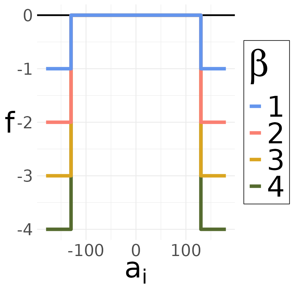
The visual field utility function attracts agents to positions in which they are able to see other group members. The idea behind this utility function is again similar to the walk beside utility function in that agents who walk together with group members like to converse with them, therefore wanting to walk besides them. The approach to generating this behavior is, however, different in the sense that for the walk beside utility function, conversing with a group member is situational while for the visual field utility function, this behavior endures throughout the complete walking trajectory.

To compute this utility function, we define the angles $a_{ij}$ from cell $i$ to the predicted position of group member $j$ and, based on these angles, define $a_i$ as the angle for which $cos\left(a_{ij}\right)$ is maximal, effectively selecting the group member who falls closest to the angle of the cone in which cell $i$ is located. Using these angles, we then define the utility function as:

$$\begin{equation} f_i = \begin{cases} 0, & \quad{\text{if $a_i$ lies in the extended visual field}} \\ -\beta, & \quad{\text{if $a_i$ does not lie in the extended visual field}} \end{cases} . \end{equation}$$

Importantly, the agent’s visual field that usually spans $[-85^\circ, 85^\circ]$ is extended by $45^\circ$ in both directions, therefore creating an extended visual field of $[-130^\circ, 130^\circ]$. The idea behind the extension is that people can turn their heads for about $45^\circ$ in both directions while talking to a group member. The effect of this utility function is displayed in the following figure:

In predped, this utility functions parameter $\beta$ is called b_visual_field.

Discussion

The M4MA’s utility framework is designed to be extensible, allowing the addition of whichever tactical choices and/or component utility functions that are required to allow the M4MA to create realistic walking behavior. The model is still under development, and so some features may change in the future. The development stage of the model may be especially visible in the component utility functions, where the boundaries between some of these seem to be blurred (e.g., visual field utility function and walk beside utility function). If you would like to help out with this development, please reach out to either Andrew Heathcote or Niels Vanhasbroeck.

It is furthermore useful to note that the M4MA is an estimable model, meaning that most (if not all) of the parameters discussed in this section can be derived based on walking data. To see how you can use predped for these types of estimations, we refer the interested reader to the vignette on Estimation.

References

Antonini, G., Martinez, S. V., Bierlaire, M., & Thiran, J. P. (2006). Behavioral priors for detection and tracking of pedestrians in video sequences. International Journal of Computer Vision, 69(2), 159-180. doi: 10.1007/s11263-005-4797-0

Campanella, M., Hoogendoorn, S. P., & Daamen, W. (2014). The Nomad model: Theory, developments and applications. Transportation Research Procedia, 2, 462-467. doi: 10.1016/j.trpro.2014.09.061

Helbing, D. & Molnár, P. (1995). Social force models for pedestrian dynamics. Physical Review E, 51(5), 4282-4286.

Hoogendoorn, S. P. & Bovy, P. H. L. (2004). Pedestrian route-choice and activity scheduling theory and models. Transportation Research Part B, 38, 169–190. doi: 10.1016/S0191-2615(03)00007-9

Larmet, V. (2022). cppRouting: Algorithms for routing and solving the traffic assignment problem. https://CRAN.R-project.org/package=cppRouting

Robin, T., Antonini, G., Bierlaire, M., & Cruz, J. (2009). Specification, estimation, and validation of a pedestrian walking behavior model. Transportation Research Part B, 43, 36-56. doi: 10.1016/j.trb.2008.06.010

Schadschneider, A., Kirchner, A., & Nishinari, K. (2002). CA approach to collective phenomena in pedestrian dynamics. Bandini, S and Chopard, B., & Tomassini, M. (Eds.), ACRI International Conference on Cellullar Automata for Research and Industry 2002. Springer-Verlag.