Advanced Simulations

In the vignette Simulations, we explained the basic workflow behind performing a simulation. In this vignette, we will dive deeper into tweaks one can do to further personalize these simulations.

Initial Conditions

Up to now, simulations have always started from scratch, having no agents inside of the environment at the start and slowly building towards a greater number of agents within the space. However, there may be occasions where the user may want to start a simulation from a particular initial condition or initial state, for example starting with $X$ number of people in the room or continuing a previous simulation from a particular iteration thereof. In this section, we will describe several ways in which users can provide initial conditions to the simulate function.

While we will only focus on the simulate function, some of the functionality underlying the creation of initial conditions is handled by a dedicated function, namely create_initial_condition. Please consult its documentation for an overview of all functionalities underlying this function.

Initial state

The most straightforward way to include an initial condition is by providing an instance of a state to the initial_condition argument in simulate, which then serves as the first state of the simulation. Assuming we have defined my_predped as an instance of the predped class, and furthermore assuming that initial_state is an instance of the state class that will serve as our initial condition, we can start the simulation from this point by calling:

trace <- simulate(
  my_predped,
  initial_condition = initial_state,
  # Additional arguments defining the simulation
)

How one comes about initial_state is left to the user, but it will most often come from a previous simulation, such as in the following example:

# Simulate an initial trace
trace <- simulate(
  my_predped,
  max_agents = 3,
  iterations = 100
)

# Continue starting from the last state in 
# this trace
my_state <- trace[[101]]
continued_trace <- simulate(
  my_predped,
  max_agents = 3,
  iterations = 100, 
  initial_condition = my_state
)

Note that providing a state to the initial_condition argument only works if both the state and the model – here, varaibles initial_state and my_predped – both contain the same environment under their slot setting. Furthermore note that the only property of the state that is retained for the new simulation is the list of agents that it contains. It may therefore be more interesting to consider the next approach for controlling initial conditions.

Initial List of Agents

A second option is to provide a list of agents that serve as the first people in the room. This list can be provided to the initial_agents argument of simulate:

# Retrieve the agents-list from an initial state
my_agents <- agents(my_state)

# Simulate using this initial list of agents
continued_trace <- simulate(
  my_predped,
  initial_agents = my_agents,
  # Additional arguments defining the simulation
)

One can also create agents manually through either their constructor agent or through the functions add_agent and add_group. This allows users to place agents at locations are deemed interesting from a simulation perspective.

Initial Number of Agents

Finally, users can let predped take care of creating an initial condition itself by specifying the initial_number_agents argument of simulate. Rather than controlling all specifics of the agents in the initial conditions, specifying this argument allows users to control only the number of agents that the simulation starts up with, letting predped take care of heterogeneity, locations, and goals:

# Start simulation with 3 agents in the room
trace <- simulate(
  my_predped,
  initial_number_agents = 3,
  # Additional arguments defining the simulation
)

Note that when the specified number of people doesn’t fit, the algorithm generating these agents will stop and provide the agents it was able to generate as an initial condition instead.

# Try to fit too many people in the room
trace <- simulate(
    my_predped,
    max_agents = 3,
    iterations = 10,
    initial_number_agents = 50
)
#> 
#> Precomputing edges
#> Your model: model vjubq is being simulated

Note that there is no guarantee that the required number of agents is generated, even when this number is realistic for the provided environment.

Precedence

It is useful to know which arguments take precedence when specifying multiple of them at once (though this is not recommended). The argument initial_agents takes precedence, followed by initial_number_agents and, finally, initial_condition.

One-directional Flow

Up to now, we have assumed pedestrian flow to be bidirectional, that is that pedestrians are able to walk in two directions across the whole environment. However, there are cases in which pedestrian flow is limited to only a single direction, which is for example the case at art exhibitions, gates at the metro station, or the one-directional aisles in the supermarkets during the COVID-19 pandemic. Given the ubiquity of unidirectional flow, we included functionalities to restrict pedestrian movement to a single direction through the definition of segments and providing them to the limited_access slot of the background class. In predped, segments are defined by their first (from) and second coordinate (to) and can be created as follows:

# Create a segment that starts at the origin and goes to coordinate P(1, 1)
my_segment <- segment(
  from = c(0, 0), 
  to = c(1, 1)
)

Providing segments to the limited_access slot will restrict access of pedestrians in such a way that they can either cross or not cross the segment itself. A visual representation of this is shown in the following figure:

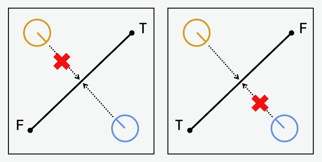
A segment going from the coordinate $F$ to another coordinate $T$ (from and to respectively) ensures an agent that stand on the left of this segment cannot cross the segment. From a mathematical viewpoint, this comes down to the following formalism: Defining $\bm{x}$ as a coordinate, defining the orientation of the segment as the angle $a_{\text{segment}} = \text{arctan}(\bm{x}_\text{to} - \bm{x}_\text{from})$, and the orientation of the agent relative to the start of the segment as $a_{\text{agent}} = \text{arctan}(\bm{x}_\text{agent} - \bm{x}_\text{from})$, then a segment restricts the agent’s movement when:

$$\begin{equation} a_{\text{agent}} - a_{\text{segment}} \in \begin{cases} [0, \pi], & \quad{\text{agent cannot cross}} \\ (\pi, 2 \pi), & \quad{\text{agent can cross}} \end{cases} \end{equation}$$

Let’s put this to practice. First, we define a simplified version of a train station where people can enter the space either through one of the entrances or through the train tracks. Such a simplified train station may look as follows:

train_station <- background(
  # Define a space of size (10, 5) meters
  shape = rectangle(
    center = c(0, 0), 
    size = c(10, 5)
  ), 
  
  # Define some gates at the entrances. These gates are 
  # not interactable.
  objects = list(
    # Gates on the left
    rectangle(
      center = c(-3, 0), 
      size = c(0.6, 1.3),
      interactable = FALSE
    ), 
    rectangle(
      center = c(-3, 1.9), 
      size = c(0.6, 1.2),
      interactable = FALSE
    ),
    rectangle(
      center = c(-3, -1.9), 
      size = c(0.6, 1.2),
      interactable = FALSE
    ),

    # Gates on the right
    rectangle(
      center = c(3, 0), 
      size = c(0.6, 1.3),
      interactable = FALSE
    ), 
    rectangle(
      center = c(3, 1.9), 
      size = c(0.6, 1.2),
      interactable = FALSE
    ),
    rectangle(
      center = c(3, -1.9), 
      size = c(0.6, 1.2),
      interactable = FALSE
    )
  ),

  # Define the entrances themselves. The two entrances
  # at the top and bottom of the space represent the 
  # stairs agents can use to exit the train tracks. 
  # The two entrances at the left and right represent
  # the entrances of the train station.
  entrance = rbind(
      # Top and bottom
      c(0, 2.5), 
      c(0, -2.5),

      # Left and right
      c(-5, 0),
      c(5, 0)
  )
)  

which when plotted gives:

plot(train_station)
#> Loading required namespace: ggplot2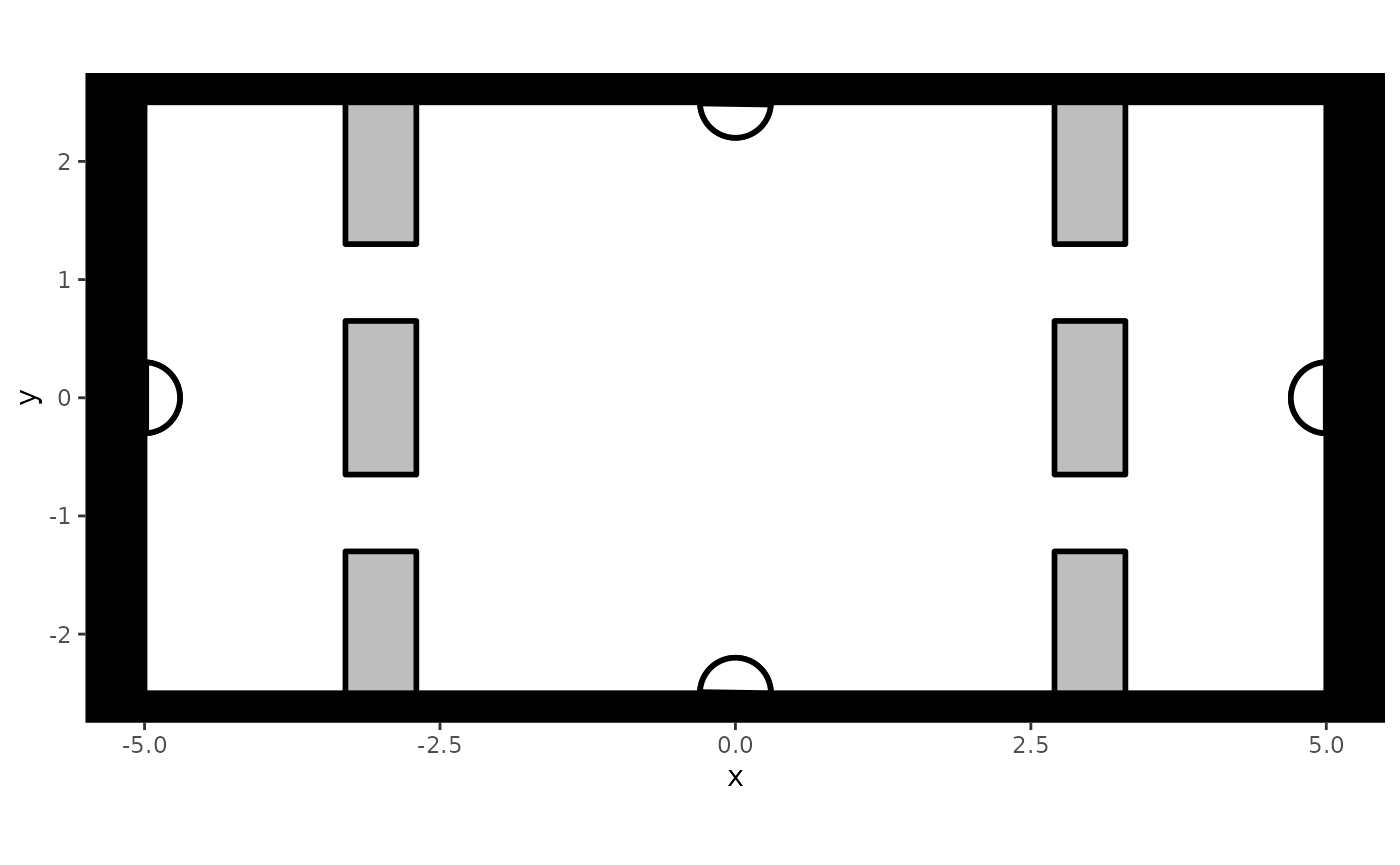

Let’s impose unidirectionality in passing through the gates, so that people always have to take the gates to their right to exit or enter the train station. To achieve this, we add segments to each of the gates as follows:

# Add segments that deal with directionality to the 
# previously defined train station
limited_access(train_station) <- list(
  # Gates on the left
  segment(from = c(-3.3, -0.6), to = c(-3.3, -1.3)),
  segment(from = c(-2.7, 0.6), to = c(-2.7, 1.3)),
  
  # Gates on the right
  segment(from = c(2.7, -0.6), to = c(2.7, -1.3)),
  segment(from = c(3.3, 0.6), to = c(3.3, 1.3))
)

We can visualize the unidirectionality by using the plot method once again:

# Plot the train station. The argument `segment.hjust` 
# makes sure arrows are plotted entirely to the left 
# of the segment, that is that the arrow's point lies 
# directly on center of the segment itself.
plot(
  train_station, 
  segment.hjust = 0
)

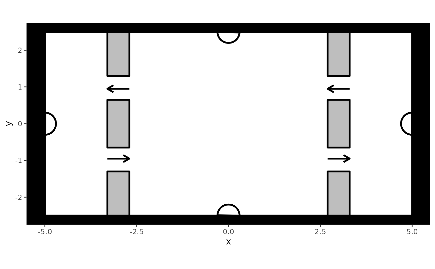
This figure again shows the train station, but includes arrows that point in the direction that agents can move into at the specified locations. Note that the segments were added at the end of the gates rather than in the middle of them: Experience teaches us that agents have the tendency to move into closed gates before realizing they are not accessible, a problem that is still under investigation.

To see unidirectionality in action, we create another instance of the predped class and simulate movement data within this restricted train station:

set.seed(1)

# Link the train station to the agent characteristics
my_predped <- predped(
  setting = train_station,
  archetypes = c(
    "BaselineEuropean", 
    "DrunkAussie"
  ), 
  weights = c(0.75, 0.25)
)

# Simulate some data
trace <- simulate(
  my_predped, 
  max_agents = 10, 
  iterations = 250,
  add_agent = 5,
  print_iteration = TRUE
)

# Visualize and turn into a GIF
plt <- plot(trace)
gifski::save_gif(
  lapply(plt, print), 
  file.path("unidirectional_example.gif"),
  delay = 1/10
)

knitr::include_graphics(
  file.path("../man/figures/unidirectional_example.gif")
)

Situational Changes

A lot of the functionality that we displayed up to now has assumed that you can prespecify the behavior of the agents, meaning you do not control the behavior of the agents once the simulation is running. Yet, the user may wish to more directly influence the course of a simulation, for example to urge pedestrians to perform an evacuation, to let agents walk around as they would in a dynamic experiment, or to adjust an agent’s parameters so that they rush to catch their train. This kind of conditional manipulations are possible in predped, specifically through the specification of the fx argument of the simulate function.

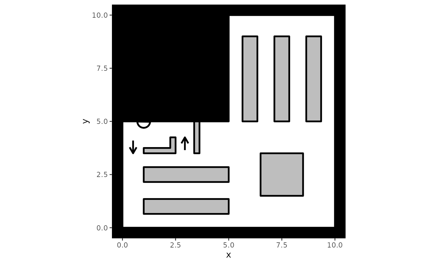
Let’s take the evacuation as an example. First, we create a simplified supermarket environment:

# Create a simplified version of a supermarket
supermarket <- background(
  # Shaking things up: Create a polygon environment
  shape = polygon(
    points = cbind(
      c(0, 0, 5, 5, 10, 10), 
      c(0, 5, 5, 10, 10, 0)
    )
  ), 

  # Objects in the environment, consisting of 
  # some shelves and a gated entrance. Gates are
  # again not interactable.
  objects = list(
    # Top shelves
    rectangle(center = c(7.5, 7), size = c(0.7, 4)),
    rectangle(center = c(6, 7), size = c(0.7, 4)),
    rectangle(center = c(9, 7), size = c(0.7, 4)),

    # Bottom shelves
    rectangle(center = c(3, 2.5), size = c(4, 0.7)),
    rectangle(center = c(3, 1), size = c(4, 0.7)),

    # Central box
    rectangle(center = c(7.5, 2.5), size = c(2, 2)),

    # Cash register and gate
    polygon(
      points = cbind(
        c(1, 2.25, 2.25, 2.5, 2.5, 1), 
        c(3.75, 3.75, 4.25, 4.25, 3.5, 3.5)
      ), 
      interactable = FALSE
    ),
    rectangle(
      center = c(3.5, 4.25), 
      size = c(0.25, 1.5), 
      interactable = FALSE
    )
  ),

  # Entrance and exit are at the cash register
  entrance = c(1, 5),

  # Limited access so that agents have to pass the cash 
  # register beforehand
  limited_access = list(
    segment(from = c(1, 3.5), to = c(0, 3.5)),
    segment(from = c(2.5, 4.25), to = c(3.375, 4.25))
  )
)

# Plot the supermarket
plot(
  supermarket, 
  segment.hjust = 1
)

Within our simulation, we want agents to enter the room, walk around to get the items they want to buy, but then be forced to evacuate at a particular time during the evacuation. To achieve this, we have to specify the fx argument, providing it with a function that takes in the state at each iteration of the simulation and allows the user to make a set of desired changes to this state. For our evacuation procedure, we create the function start_evacuation, starting an evacuation after 100 iterations:

start_evacuation <- function(state) {
  # Check whether the current iteration is greater than 
  # 100. If not, then we do not want to change the state.
  if(iteration(state) == 100) {
    # Delete all agents that were waiting to enter the
    # space.
    potential_agents(state) <- list()

    # Delete all goals of the agents that are running 
    # around in the supermarket. This pertains to both
    # the goal list and the current goal
    for(i in seq_along(agents(state))) {
      # Extract this agent
      agent_i <- agents(state)[[i]]

      # Change their current activities
      goals(agent_i) <- list()
      current_goal(agent_i)@counter <- 0
      status(agent_i) <- "completing goal"

      # Put the agent back in the list
      agents(state)[[i]] <- agent_i
    }

    # Make sure that agents cannot be added anymore
    # by lowering the maximal number of agents to 0
    iteration_variables(state)$max_agents <- 0
  }

  return(state)
}

Several things in this function deserve note:

• A conditional statement in this function checks for the iteration number in the simulation, ensuring that the evacuation procedure only starts when $100$ iterations have passed;
• Within the if-statement, we adjust the state so that the evacuation can start. Specifically, we make the following changes:
  • We ensure no agents are standing in line, waiting to enter the space (delete the contents of the potential_agents slot);
  • We ensure the space should be empty by setting max_agents to $0$ in the iteration_variables;
  • We adjust the agents so that they have no more goals to achieve, triggering them to leave the environment.

With this function defined, we can now run the simulation:

set.seed(1)

# Connect environment to agent characteristics
my_predped <- predped(
    setting = supermarket, 
    archetypes = "BaselineEuropean"
)

# Run the simulation and provide our function 
# to the `fx` argument
trace <- simulate(
    my_predped, 
    max_agents = 30, 
    add_agent = 5, 
    iterations = 250, 
    fx = start_evacuation
)

# Create plots and GIF
plt <- plot(
    trace, 
    segment.hjust = 1
)

# Provide a cue of when the evacuation starts
plt[[101]] <- plot(
  trace[[101]], 
  segment.hjust = 1,
  shape.fill = "red"
)

# Save to a gif
gifski::save_gif(
    lapply(plt, print),
    file.path("supermarket.gif"),
    delay = 1/10
)

Of course, you are not limited to changing the agents, but can also change the environment itself. For example, if we want to allow agents to ignore the unidirectionality imposed at the beginning of the simulation, we can empty the limited_access slot once the evacuation has started:

start_evacuation <- function(state) {
  if(iteration(state) == 100) {
    potential_agents(state) <- list()
    
    for(i in seq_along(agents(state))) {
      agent_i <- agents(state)[[i]]
      
      goals(agent_i) <- list()
      current_goal(agent_i)@counter <- 0
      status(agent_i) <- "completing goal"

      agents(state)[[i]] <- agent_i
    }

    iteration_variables(state)$max_agents <- 0

    # Delete the limited access
    limited_access(state@setting) <- list()
  }

  return(state)
}

In other words, the fx argument allows users to create a whole range of situations that go beyond the simple “walk around and attain a set of goals”, including evacuations, experimental designs, peak and off-peak densities, and many more situations without having to worry about the implementational details of the package.

Bookkeeping through the variables Slot

If one wants to create even more complicated situations, one can leverage the variables slot of the state class to make bookkeeping across the simulation easier. This slot keeps hold of a named list containing all variables relevant to your simulation. Keeping within our evacuation example, we may want to keep track of how long it takes each agent to leave the room after the evacuation has been signalled. We can achieve this by creating a variables of times in the variable slot and updating it accordingly, for example redefining start_evacuation as:

start_evacuation <- function(state) {
  # Ensures the start of the evacuation and creates the variable of interest
  if(iteration(state) == 100) {
    potential_agents(state) <- list()
    
    for(i in seq_along(agents(state))) {
      agent_i <- agents(state)[[i]]
      
      goals(agent_i) <- list()
      current_goal(agent_i)@counter <- 0
      status(agent_i) <- "completing goal"

      agents(state)[[i]] <- agent_i
    }

    iteration_variables(state)$max_agents <- 0

    # Create the times variable as a vector of 0s of the same length as the 
    # agents, containing their names
    variables(state)$times <- numeric(length(agents(state))) |>
      `names<-` (sapply(agents(state), id))
  }

  # Update the variables based on who is leaving the simulation
  if(iteration(state) > 100) {
    # Extract the times 
    times <- variables(state)$times 

    # Check whether any agent has left the simulation
    ids <- sapply(
      agents(state),
      id
    )
    left <- !(names(times) %in% ids) & times == 0

    # Update the times and put back in the list
    times[left] <- iteration(state) - 100
    variables(state)$times <- times
  }

  return(state)
}

We can then rerun the simulation using the code above and inspect the resulting evacuation times by extracting the variable from the final iteration:

#> 
#> Precomputing edgesYour model: model ydgab is being simulated

variables(trace[[251]])$times
#> donzm eyqaz llyry mvzfl owfjm rbnvd kheaq oggxf dobyg senmi wvijj iypko 
#>    67    23    98   113    47    80   102    19    93    41     6     3

Using your Own Parameters

While we provide a lot of prespecified agent types to choose from, one may wish to play around with the parameters themselves to personalize their own simulations. In this case, one may wish to save the parameters for future use. In this case, you can let the predped constructor know what parameters you would want to use by specifying the filename argument:

my_predped <- predped(
  setting = my_background, 
  filename = file.path("path", "to", "file")
)

The typical workflow for using your own parameters is thus the following:

• Load the default parameters of predped;
• Adjust the parameters of interest;
• Save them in a separate file;
• Link to this file when you create an instance of the predped class.

In code, this workflow looks like this:

# Read in default parameters
params <- load_parameters()

# Only retain the BaselineEuropean in the parameters and 
# change their preferred speed to 0.5 m/s
means <- params[["params_archetypes"]]
params[["params_archetypes"]] <- means |>
  # Only retain BaselineEuropean
  dplyr::filter(name == "BaselineEuropean") |>

  # Change preferred speed
  dplyr::mutate(preferred_speed = 0.5)

# Also change params_sigma to only retain the 
# BaselineEuropean
covariances <- params[["params_sigma"]]
params[["params_sigma"]] <- covariances["BaselineEuropean"]

# Save this list of parameters in a local file
saveRDS(
  params, 
  file.path("my_parameters.Rds")
)

# Create an instance of the predped class
my_predped <- predped(
  setting = my_background, 
  filename = file.path("my_parameters.Rds")
)

In this example, we saved the complete parameter list in one .Rds file, but one can also choose to only adjust one part of this list and combine it with the defaults of the package. For example, we can change and save "params_archetypes" and read it in through the predped constructor:

# Read in default parameters
params <- load_parameters()

# Only retain the BaselineEuropean in the parameters and 
# change their preferred speed to 0.5 m/s
means <- params[["params_archetypes"]]
means <- means |>
  # Only retain BaselineEuropean
  dplyr::filter(name == "BaselineEuropean") |>

  # Change preferred speed
  dplyr::mutate(preferred_speed = 0.5)

# Save the means as a separate data.frame
write.table(
  means, 
  file.path("my_parameters.csv")
)

# Read in these parameters through predped
my_predped <- predped(
  setting = my_background, 
  filename = file.path("my_parameters.csv"),
  sep = " "
)

Note that the sep argument denotes the delimiter that is used in the saved file. Furthermore note that the file has been merged with the predped defaults, and that parameters(my_predped) still returns a list containing the three slots mentioned earlier.

Similar to the case with only one slot of the list, predped can also deal with changes in a few components in a list, as long as they are saved in a list with the correct slot names:

# Read in default parameters
params <- load_parameters()

# Only retain the BaselineEuropean in the parameters and 
# change their preferred speed to 0.5 m/s
means <- params[["params_archetypes"]]
means <- means |>
    # Only retain BaselineEuropean
    dplyr::filter(name == "BaselineEuropean") |>
    # Change preferred speed
    dplyr::mutate(preferred_speed = 0.5)

# Also change params_sigma to only retain the 
# BaselineEuropean
covariances <- params[["params_sigma"]]
covariances <- covariances["BaselineEuropean"]

# Make a new parameter list and save it
new_parameters <- list(
    "params_archetypes" = means, 
    "params_sigma" = covariances
)
saveRDS(new_parameters, file.path("my_parameters.Rds"))

# Read in these parameters through predped
my_predped <- predped(
    setting = my_background, 
    filename = file.path("my_parameters.Rds")
)

Note that if the content of a slot in the list does not have the same structure as the original parameters, predped will provide an error. If the name of the slot itself does not correspond to the original, it will discard the content and replace it with the defaults.