Adding noise

The first important functionality of the package is to add noise to positional data. This is a useful feature when setting up parameter recovery studies, especially if one wants to preserve some type of “realism” in these studies. The primary function to “noise up” the data is noiser, the functionality of which will be explained in this section.

Measurement model

When you add noise to (simulated) positional data, you implicitly assume that there is a difference between the measurement of a position and the actual (latent) position. Within the package, the function that connects the measurement to the latent position is called the measurement model, which can be written down as:

$$\begin{equation} \mathbf{y} = \mathbf{f}(\mathbf{x}) \end{equation}$$ where $\mathbf{y}$ represents the measurement of the latent position $\mathbf{x}$. In other words, the measurement depends on but is not equal to the latent position. How exactly these two relate depends on the link function $\mathbf{f}$, two of which are implemented in the package.

Independent error

With independent error, we mean that the error added to the latent position is (a) independent of the process itself (i.e., independent of the value of $\bm{x}$) and (b) independent of time. One example of a measurement model in which this is the case is the following.

Denote $\bm{y}_i$ as the measurement taken at time $t_i$, and furthermore denote $\bm{x}_i$ as the latent position at that same time, then condition (a) is met if we define the relationship between $\bm{y}_i$ and $\bm{x}_i$ as:

$$\begin{equation} \bm{y}_i = \bm{x}_i + \bm{\epsilon}_i \end{equation}$$ where $\bm{\epsilon}$ represents the associated measurement error. Importantly for condition (a), $\bm{\epsilon}$ is independent of $\bm{x}$, meaning that the observation or measurement $\bm{y}$ can be obtained through a simple adding of the error to the process, without any interactions between both components. This assumption conforms to the classical measurement theory perspective (Lord et al., 1968) and will be assumed throughout.

What’s left is to defined $\bm{\epsilon}$. Conforming to condition (b), we assume that $\bm{\epsilon}$ is drawn from a multivariate normal distribution so that:

$$\begin{equation} \bm{\epsilon} \overset{iid}{\sim} N(\bm{\mu}, \Sigma) \end{equation}$$ where $\bm{\mu}$ represents the mean of the error (e.g., in case there is bias) and $\Sigma$ is the covariance matrix of the error.

Temporal error

With temporal error, we mean that the error added to the latent position is (a) independent of the process itself and (b) depends on time. This means that we still conform to the previously defined relationship between $\bm{y}$ and $\bm{x}$, so that:

$$\begin{equation} \bm{y}_i = \bm{x}_i + \bm{\epsilon}_i \end{equation}$$ However, our model of $\bm{\epsilon}$ changes. Within the package, we assume that the error changes over time as a vector autoregressive process, so that:

$$\begin{equation} \bm{\epsilon}_i = \bm{\delta} + \Theta \bm{\epsilon}_{i - 1} + \bm{\omega}_i \end{equation}$$ where $\bm{\epsilon}_i$ represents the measurement error at time $t_i$, $\bm{\delta}$ is the intercept of the (measurement) process, $\Theta$ is the transition matrix, defining the linear temporal structure of the error, and $\bm{\omega}_i$ is the innovation of the measurement process at time $t_i$ (Hamilton, 1994). The innovations themselves are distribution according to a multivariate normal distribution, so that:

$$\begin{equation} \bm{\omega} \overset{iid}{\sim} N(\bm{0}, \Sigma) \end{equation}$$ where $\Sigma$ is the covariance matrix of the innovations.

If you were to specify the parameters of this model, it is useful to keep the take the first moments of $\bm{\epsilon}$ according to the vector autoregressive model into account, especially if one wishes to relate these to the independent error model. According to the vector autoregressive model, the mean $\bm{\mu}$ and covariance $\Sigma_\epsilon$ of $\bm{\epsilon}$ are equal to:

$$\begin{equation} \bm{\mu} = (I - \Theta)^{-1} \bm{\delta} \end{equation}$$

$$\begin{equation} \Sigma_\epsilon = \Sigma - \Theta \Sigma \Theta^T \end{equation}$$ where $I$ is the identity matrix.

Using noiser

With the mathematics out of the way, we can now focus on how to use the noiser function itself to achieve the wanted results. First, we generate a dataset called data displaying circular motion.

# Define the simulated angles of the observations
angles <- seq(0, 2 * pi, length.out = 50)

# Define the dataset itself
data <- data.frame(
  time = 1:50, 
  x = 10 * cos(angles),
  y = 10 * sin(angles)
)

# Plot these data
plot(data$x, data$y)

Latent positions on a plane representing circular motion.

Once these data have been created, we can add noise to them through the noiser function. Using the independent measurement model with mean $\bm{\mu} = \begin{bmatrix} 1 \\ 1 \end{bmatrix}$ and $\Sigma = \begin{bmatrix} 1 & 0.25 \\ 0.25 & 1 \end{bmatrix}$ for this purpose can be achieved through calling the following code:

# Add noise to the data
noised_up <- noiser(
  data, 
  model = "independent",
  mean = c(5, 5),
  covariance = c(1, 0.25, 0.25, 1) |>
    matrix(nrow = 2, ncol = 2)
)

# Plot the noised up data
plot(noised_up$x, noised_up$y)

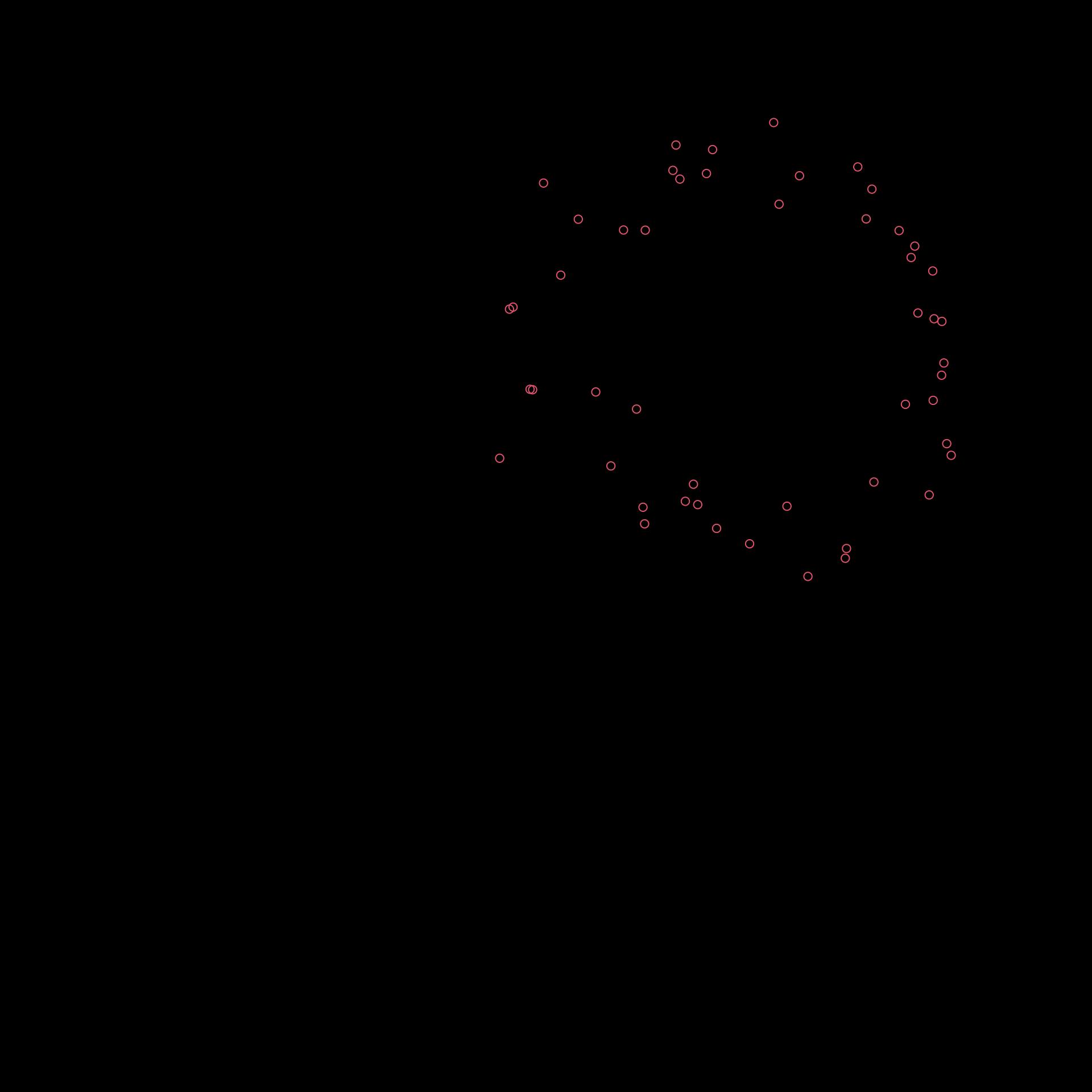
Measured positions on a plane representing circular motion. Error was added according to the independent measurement model.

Notice that due to the specification of $\bm{\mu}$, the noisy data have been moved to fall around this new mean.

Using the temporal model can be achieved in a similar way. Specifying $\bm{\delta} = \begin{bmatrix} 2.5 \\ 2.5 \end{bmatrix}$, $\Theta = \begin{bmatrix} 0.5 & 0 \\ 0 & 0.5 \end{bmatrix}$, and $\Sigma = \begin{bmatrix} 1.33 & 0.33 \\ 0.33 & 1.33 \end{bmatrix}$, so that $\bm{\mu} = \begin{bmatrix} 1 \\ 1 \end{bmatrix}$ and $\Sigma_\epsilon = \begin{bmatrix} 1 & 0.25 \\ 0.25 & 1 \end{bmatrix}$, we write:

# Add noise to the data
noised_up <- noiser(
  data, 
  model = "temporal",
  intercept = c(2.5, 2.5),
  transition = diag(2) * 0.5,
  covariance = c(4/3, 1/3, 1/3, 4/3) |>
    matrix(nrow = 2, ncol = 2)
)

# Plot the noised up data
plot(noised_up$x, noised_up$y)

Measured positions on a plane representing circular motion. Error was added according to the temporal measurement model.

Things to look out for

When specifying the parameters of the measurement models, there are several things that you should look out for. First, one should closely consider the dimensionality of the parameters when specifying them. Specifically, the denoiser package works on the assumption that things have been measured/simulated on two-dimensional plane, meaning that all data should consist of an x- and y-coordinate. The parameters provided to the native independent and temporal models should cohere to this specification. This means that, for the independent model, the mean should consist of exactly 2 values and the covariance should consist of a $2 \times 2$ matrix. While noiser can handle deviations in this specification for the mean, it cannot do so for the covariance:

# Specify only one mean: In this case, the value is used for both dimensions
noised_up <- noiser(
  data, 
  model = "independent",
  mean = 5,
  covariance = diag(2)
)
head(noised_up)

##   time        x         y
## 1    1 15.83021  4.570620
## 2    2 15.42149  7.639233
## 3    3 15.86659  7.465688
## 4    4 15.02089  8.480516
## 5    5 12.25735  7.460495
## 6    6 13.84274 11.046592

# Specify three means: In this case, only the first two values are used
noised_up <- noiser(
  data, 
  model = "independent",
  mean = c(5, 10, 15),
  covariance = diag(2)
)
head(noised_up)

##   time        x         y
## 1    1 15.57895  9.643876
## 2    2 15.06333 10.214307
## 3    3 14.14649 13.613662
## 4    4 12.53559 14.934246
## 5    5 12.26453 15.105568
## 6    6 11.49594 15.580700

# Specify a 1D matrix for the covariances: Leads to an error
noised_up <- noiser(
  data, 
  model = "independent",
  mean = c(5, 5),
  covariance = diag(1)
)

## Error in `measurement_models[[model]]()`:
## ! Provided covariance matrix does not have the right dimensionality. A 1 x 1 matrix is provided instead of the required 2 x 2 matrix.

# Specify a 3D matrix for the covariances: Leads to an error
noised_up <- noiser(
  data, 
  model = "independent",
  mean = c(5, 5),
  covariance = diag(3)
)

## Error in `measurement_models[[model]]()`:
## ! Provided covariance matrix does not have the right dimensionality. A 3 x 3 matrix is provided instead of the required 2 x 2 matrix.

Similar restrictions for the parameters hold for intercept, transition, and covariance for the temporal model, where transition and covariance should both be $2 \times 2$ matrices. Like for the independent measurement model, noiser is robust against misspecification of the dimension for the intercept, but not for transition and covariance.

Second, when specifying the covariance matrix, one should ensure that it is positive definite. This means that (a) its eigenvalues should be positive, (b) it should be a symmetric matrix, and (c) it is not reducable in dimensionality (i.e., its leading minors should be positive). Examples on non-positive-definite matrices are the following:

# Negative eigenvalues
noised_up <- noiser(
  data, 
  model = "independent",
  mean = c(0, 0),
  covariance = diag(2) * (-1)
)

## Error in `MASS::mvrnorm()`:
## ! 'Sigma' is not positive definite

# Negative eigenvalues
noised_up <- noiser(
  data, 
  model = "independent",
  mean = c(0, 0),
  covariance = c(1, 2, 2, 1) |>
    matrix(nrow = 2, ncol = 2)
)

## Error in `MASS::mvrnorm()`:
## ! 'Sigma' is not positive definite

# Reducable in dimension: Note that no error is thrown!
noised_up <- noiser(
  data, 
  model = "independent",
  mean = c(0, 0),
  covariance = c(1, 0, 0, 0) |>
    matrix(nrow = 2, ncol = 2)
)

An easy way to ensure the covariance matrix is positive definite is by specifying it’s Cholesky decomposition instead. Specifically, any positive definite matrix can be decomposed so that:

$$\begin{equation} \Sigma = \Gamma \Gamma^T \end{equation}$$ where for $\text{dim}(\Sigma) = 2 \times 2$, $\Gamma$ is:

$$\begin{equation} \Gamma = \begin{bmatrix} \gamma_1 & 0 \\ \gamma_{12} & \gamma_{2} \end{bmatrix} \end{equation}$$

By specifying the matrix $\Gamma$ instead of $\Sigma$, one therefore ensures that noiser can run. Note, however, that this doesn’t ensure that the results make sense: This is up for the user to decide.

An example of how one can use the Cholesky decomposition instead of specifying $\Sigma$ directly:

# Define the lower-triangular Cholesky matrix based on random numbers. Maximal standard deviation/covariance of 1
gamma <- runif(3, min = 1e-2, max = 1)
G <- c(gamma[1], gamma[2], 0, gamma[3]) |>
  matrix(nrow = 2, ncol = 2)

# Create the covariance matrix
S <- G %*% t(G)

# Use noiser to add noise to the data
noised_up <- noiser(
  data, 
  model = "independent",
  mean = c(0, 0),
  covariance = S
)

# Plot the noised up data
plot(noised_up$x, noised_up$y)

Measured positions on a plane representing circular motion. Error was added according to the independent measurement model with a randomly generated covariance matrix through its Cholesky decomposition.

Nonstandard column names

Up to now, our data has consisted of three columns, namely time, x, and y. This is the data structure that is expected by the functions in the denoiser package. If your data does not conform to this structure and you wish to use the noiser function, the function will automatically throw an error:

# Create data with nonstandard column names
angles <- seq(0, 2 * pi, length.out = 50)

data <- data.frame(
  seconds = 1:50, 
  X = 10 * cos(angles),
  Y = 10 * sin(angles)
)

# Add noise to these data with the defaults on
noised_up <- noiser(data)

## Error in `[.data.frame`:
## ! undefined columns selected

There are two ways around this issue. First, one can change the column names in their dataset manually so that they conform to the requirements of the functions in the package. While this is an easy way around it, it also seems lazy on the end of the developer to not include robustness against such a clear issue. We would agree with this conclusion. The second way around this issue is therefore to specify the cols argument in noiser. This argument provides a mapping of the column names that are used internally in the denoiser package to the column names that were originally present in the data through a named vector. Specifically, one can call:

# Define the mapping of the columns
mapping <- c(
  "time" = "seconds",
  "x" = "X",
  "y" = "Y"
)

# Add noise to the data through using the mapping
noised_up <- noiser(
  data, 
  cols = mapping
)
head(noised_up)

##   seconds         X            Y
## 1       1 10.008332 -0.001464746
## 2       2  9.934924  1.231661005
## 3       3  9.680141  2.485432030
## 4       4  9.272046  3.718075756
## 5       5  8.686468  4.858085884
## 6       6  7.976029  5.940597542

Note that when the data contains additional columns, that one should specify this in the cols argument.

# Create data with nonstandard column names and additional variables
angles <- seq(0, 2 * pi, length.out = 50)

data <- data.frame(
  seconds = 1:50, 
  X = 10 * cos(angles),
  Y = 10 * sin(angles),
  variable_1 = 1:50,
  variable_2 = rep("test", 50)
)

# Define the mapping of the columns
mapping <- c(
  "time" = "seconds",
  "x" = "X",
  "y" = "Y"
)

# Add noise to these data with the columns being provided
noised_up <- noiser(
  data, 
  cols = mapping
)
head(noised_up)

##   seconds        X           Y
## 1       1 9.989030 0.003668147
## 2       2 9.920981 1.320289871
## 3       3 9.689500 2.561860470
## 4       4 9.290149 3.784864101
## 5       5 8.725190 4.918384702
## 6       6 8.027195 5.978526066

# Mention the additional columns explicitly in the mapping
mapping <- c(
  "time" = "seconds",
  "x" = "X",
  "y" = "Y",
  "v1" = "variable_1",
  "v2" = "variable_2"
)

# Add noise to these data with the columns being provided
noised_up <- noiser(
  data, 
  cols = mapping
)
head(noised_up)

##   seconds         X          Y variable_1 variable_2
## 1       1 10.014854 0.01106708          1       test
## 2       2  9.903151 1.29462608          2       test
## 3       3  9.651743 2.55067656          3       test
## 4       4  9.254979 3.74998115          4       test
## 5       5  8.708365 4.92558443          5       test
## 6       6  8.012217 5.97988395          6       test

Grouping

Up to now, we have only considered adding noise for a particular dataset with only one type of movement. Imagine, however, that our dataset contains the movement of more than one individual, such as in the following case:

# Define the angles
angles <- seq(0, 2 * pi, length.out = 50)

# Create data for two participants, each walking in a circle but a few meters away from each other
data_1 <- data.frame(
  seconds = 1:50, 
  X = 10 * cos(angles),
  Y = 10 * sin(angles),
  person = 1
)
data_2 <- data.frame(
  seconds = 1:50,
  X = 5 * cos(angles) + 5,
  Y = 5 * sin(angles) + 5,
  person = 2
)
data = rbind(data_1, data_2)

# Plot these data
plot(
  data$X, 
  data$Y,
  col = factor(data$person)
)

Latent positions on a plane representing circular motion of two different people.

If one wished to add noise to these type of data, one should consider the person that generated those data in the first place. To ensure noiser generates noise while accounting for the individual, one should provide the relevant column to the .by argument, so that:

# Mention the additional columns explicitly in the mapping
mapping <- c(
  "time" = "seconds",
  "x" = "X",
  "y" = "Y"
)

# Add noise to these data with the columns being provided
noised_up <- noiser(
  data, 
  cols = mapping,
  .by = "person",
  model = "independent",
  mean = c(0, 0),
  covariance = diag(2) * 0.5
)

# Plot the result
plot(
  noised_up$X, 
  noised_up$Y,
  col = factor(noised_up$person)
)

Measured positions on a plane representing circular motion of two different people after adding noised for each person separately.

Note that you don’t have to specify the mapping of the person column when it is specified through the .by argument: This is automatically accounted for under the hood.

Specifying your own measurement model

It is possible to specify your own measurement model and provide it to noiser to noise up the data. Imagine, for example, that you would like to create your own independent measurement model, but one that depends only on a user-provided triangular matrix $\Gamma$ rather than a covariance matrix $\Sigma$, then one can do so by specifying:

# Create your own measurement model function
my_model <- function(
  data, 
  mean, 
  cholesky
) {
  # Compute the covariance matrix
  sigma <- cholesky %*% t(cholesky)

  # Use mvrnorm to generate residuals
  residuals <- MASS::mvrnorm(nrow(data), mu = mean, Sigma = sigma)

  # Add the residuals to the data
  data[, c("x", "y")] <- data[, c("x", "y")] + residuals

  return(data)
}

# Use noiser to add noise to the data
noised_up <- noiser(
  data, 
  cols = mapping,
  .by = "person",
  model = my_model,
  mean = c(0, 0),
  cholesky <- c(1, 0.25, 0, 1) |>
    matrix(nrow = 2, ncol = 2)
)

# Plot these data
plot(
  noised_up$X, 
  noised_up$Y,
  col = factor(noised_up$person)
)

Measured positions on a plane representing circular motion of two different people after adding noised for each person separately through our own measurement model.

Several things are of note here. First, my_model should make use of denoiser’s internal column names rather than the user-defined columns for the data. This means that the time variable is stored under time and the x- and y-coordinates are stored under x and y respectively. Second, one should not worry about the .by argument when specifying my_model: This is handled automatically by noiser. Finally, one can specify their own arguments in my_model and provide values to these arguments in noiser itself. As can be seen in this chunk of code, the arguments mean and cholesky of my_model are provided to noiser rather than to my_model itself: noiser will automatically provide these arguments to my_model unless otherwise specified.

Through this framework, users are able to specify their own measurement models as they please, allowing them to surpass what is provided in the package itself.

References

Hamilton, J. D. (1994). Time series analysis. Princeton University Press. doi: 10.2307/j.ctv14jx6sm

Lord, F. M., Novick, M. R., & Birnbaum, A. (1968). Statistical theories of mental test scores. Addison-Wesley.