Filtering data

The second important functionality of the package is to filter positional data to get rid of the noise inherent to these data. This is a useful feature both when setting up parameter recovery studies and when trying to analyze your own positional data. The primary function to use when filtering data is denoiser, the functionality of which will be explained in this vignette.

Filters

The denoiser function makes use of two types of filters that one can use and that have been proven (somewhat) effective when dealing with positional data. These two filters are the Kalman filter and a binning of the data, both of which will be described separately.

Kalman filter

The Kalman filter is a popular filtering technique often encountered in time-series modeling or the modeling of movement to retrieve latent states of the variables you are interested in while accounting for the properties of the measurements. Central to the Kalman filter is the definition of a movement equation and a measurement equation, the former of which defines how we expect the latent state to change over time and the latter of which defines how the measurements or observations should be related to these latent states (see again Adding noise). The definition of the movement equation can be achieved through specifying the parameters of the following equation:

$$\begin{equation} \bm{x}_i = F \bm{x}_{i - 1} + B \bm{u}_i + \bm{\epsilon}_{i} \end{equation}$$ where $\bm{x}_i$ contains the values of the relevant latent variables at time $t_i$, $F$ is the matrix relating values of these latent variables at a previous time point to the next one, $B$ is a matrix that scales the values of exogeneous inputs $\bm{u}$, and $ represents noise at the latent level. Similarly, the measurement equation can be defined through specifying the parameters of the following equation:

$$\begin{equation} \bm{z}_i = H \bm{x}_i + \bm{y}_i \end{equation}$$ where $H$ is the measurement matrix, relating the observed states $\bm{z}$ to the latent state $\bm{x}$, and where $\bm{y}$ represents the innovation, that is the part that is not captured by accounting for the latent state and should, in theory, contain the measurement error.

Note that in these equations, I deviate from the mathematical conventions used in the other vignettes. This is to align myself with the literature around the Kalman filter, making it easier for those not familiar with the Kalman filter to inform themselves when diving in the literature.

Three-step procedure

Once the parameters are defined, then the Kalman filter attempts to recover the underlying process $\bm{x}$ through filtering each observation $\bm{z}$ using a three-step procedure.

Prediction step

In the first step, the Kalman filter will use the movement equation to predict the next value of $\bm{x}$ based on its previous value. In equations:

$$\begin{equation} \bm{x}_i = F \bm{x}_{i - 1} + B \bm{u}_i \end{equation}$$ This serves as the point prediction of $\bm{x}_i$ at time $t_i$. However, the Kalman filter also accounts for the certainty of this prediction, which it computes as:

$$\begin{equation} P_i = F P_{i - 1} F^T + W \end{equation}$$ where $P_{i - 1}$ is the prior certainty matrix set around the initial condition $\bm{x}_{i - 1}$. If $i = 1$, then this represents the prior covariance $P_0$ and prior expectation $\bm{x}_0$, which should be specified by the user. If $i > 1$, then these represent the previously computed (and updated) values of $\bm{x}$ and $P$.

In this equation, $W$ represents the innovation covariance matrix, that is the covariance around $\bm{\epsilon}$ specified in the movement equation. It is assumed that:

$$\begin{equation} \bm{\epsilon} \overset{iid}{\sim} N(\bm{0}, W) \end{equation}$$ Similar to the initial conditions of $\bm{x}$ and $P$, the value of $W$ should also be provided by the user.

Once the prediction $\bm{x}_i$ and its certainty $P_i$ have been computed, we can move on to the next step of the Kalman filter.

Innovation step

In the second step, we use the measurement equation to find out how close our prediction $\bm{x}_i$ lies to the actual observation $\bm{z}_i$. Specifically, we compute the innovation $\bm{y}_i$ as:

$$\begin{equation} \bm{y}_i = \bm{z}_i - H \bm{x}_i \end{equation}$$ Similar to the prediction step, we again which to quantify the certainty around this innovation, which we achieve through computing its covariance matrix $\Sigma_i$:

$$\begin{equation} \Sigma_i = H P_i H^T + R \end{equation}$$ where $R$ is the measurement covariance matrix, representing the covariance of the measurement error. Like for the values of $\bm{x}_0$, $\bm{P}_0$, and $W$, the values in $R$ should also be provided by the user.

An important realization that we should have at this point is that we have quantified not only the certainty around our prediction through $P_i$, but also around the process in full through $\Sigma_i$. Putting these two covariance matrices against each other therefore provides us with something of a reliability measure: How much can we trust our measurements over our predictions and vice-versa, and which of the two should we trust when estimating the latent values $\bm{x}$? This is exactly what is achieved when computing the Kalman gain, which is defined as:

$$\begin{equation} K_i = P_i H^T \Sigma_i^{-1} \end{equation}$$ which will play an important role in updating our estimate of the latent process $\bm{x}$ based on the movement and measurement equations.

Updating step

The final step consists of estimating the values of the latent process $\bm{x}_i$ and the certainty around this estimate $\bm{P}_i$. This is achieved through the following set of equations, each of which concerns a weighted sum of the prediction according to the movement equation and the observation according to the measurement equation. The Kalman gain $K$ represents the weights that determine the strength of the prediction versus the observation, again basing this weight on the presumed amount of information either the observation or the prediction hold.

$$\begin{equation} \hat{\bm{x}}_i = \bm{x}_i + K \bm{y}_i \end{equation}$$

$$\begin{equation} \hat{P}_i = (I - K H) P_i \end{equation}$$ where $I$ is the identity matrix.

This concludes the three-step procedure of the Kalman filter, after which it will move to the prediction step for the next datapoint $\bm{x}_{i + 1}$ at the next time point $t_{i + 1}$. In this prediction step, the estimated values $\hat{\bm{x}}_i$ and $\hat{P}_i$ serve as the initial conditions.

Kalman models

Up to now, the discussion has been quite vague: It has specified how the Kalman filter works without going into details of what each of its parameters represents. The strength of the Kalman filter is exactly this generality. It works for any set of movement and measurement equations that can fit within the general structure outlined above. As to how to define these equations, that’s left up to the user.

Within the denoiser package, we specify only a single set of movement and measurement equations that are used to filter the data. This model is called the constant velocity model, reflecting its underlying assumption that the subject is moving at constant velocity, meaning changes in acceleration are taken as part of the measurement error. This model was used in our previous project and has been found to be (somewhat) effective at handling the measurement error observed in our experiments, which is why it is included here.

In this vignette, I will focus mostly on the definition of the parameters rather than the reasoning behind the model. For this, I refer the interested reader to the explanation of the constant_velocity function instead.

Constant velocity model

The constant velocity model operates under the assumption that the latent position changes in the following way:

$$\begin{equation} \begin{bmatrix} x \\ y \end{bmatrix}_i = \begin{bmatrix} x \\ y \end{bmatrix}_{i - 1} + \begin{bmatrix} v_x \\ v_y \end{bmatrix} \Delta t \end{equation}$$ where $v_x$ and $v_y$ represent the speed in dimensions x and y, and where $\Delta t$ represents the time interval between observations. Under this specification, we have to define the latent state $\bm{x}$ as a four-dimensional vector, taking into account both position and speed so that:

$$\begin{equation} \bm{x}_i = \begin{bmatrix} x \\ y \\ v_x \\ v_y \end{bmatrix}_i \end{equation}$$

For the movement equation, we then have to define the four-dimensional matrix $F$ and $W$, both of which depend on time interval $\Delta t$, so that:

$$\begin{equation} F_i = \begin{bmatrix} 1 & 0 & \Delta t & 0 \\ 0 & 1 & 0 & \Delta t \\ 0 & 0 & 1 & 0 \\ 0 & 0 & 0 & 1 \end{bmatrix}_i \end{equation}$$

$$\begin{equation} W_i = \begin{bmatrix} \Delta t^2 \sigma_{v_x}^2 & 0 & \Delta t \sigma_{v_x}^2 & 0 \\ 0 & \Delta t^2 \sigma_{v_y}^2 & 0 & \Delta t \sigma_{v_y}^2 \\ \Delta t \sigma_{v_x}^2 & 0 & \sigma_{v_x}^2 & 0 \\ 0 & \Delta t \sigma_{v_y}^2 & 0 & \sigma_{v_y}^2 \end{bmatrix}_i \end{equation}$$ Notice that if you fill compute $F_i \bm{x}_{i - 1}$, you will get back the original equation for $x$ and $y$, showing that these parameters do indeed conform to our assume movement equation. Furthermore note that $W_i$ can be obtained by assuming some error on the speed variables $v_x$ and $v_y$ and, similarly, working this out according to the movement equation denoted above.

For the measurement equation, we have to define the measurement matrix $H$ which connects the underlying latent movement model and the observations that we make. In denoiser, we assume that we only measured positions without any indication of speeds, meaning that our measurement matrix $H$ will have to reduce information so that:

$$\begin{equation} H = \begin{bmatrix} 1 & 0 & 0 & 0 \\ 0 & 1 & 0 & 0 \end{bmatrix} \end{equation}$$ Again notice that using this measurement matrix on the previously computed values of $F_i \bm{x}_{i - 1}$, you will automatically get back the movement equation denoted above in terms of $x$ and $y$.

On the level of the measurement equation, we also have to define the measurement covariance matrix R, which for our purposes is defined as:

$$\begin{equation} R = \begin{bmatrix} \sigma_R^2 & 0 \\ 0 & \sigma_R^2 \end{bmatrix} \end{equation}$$

In its current specification, there are still several parameters that need to be specified by the user. This includes the initial conditions $\bm{x}_0$ and $P_0$, the measurement variance $\sigma_R^2$, and the movement variances $\sigma_{v_x}^2$ and $\sigma_{v_y}^2$.

In denoiser, we specify broad though data-driven priors. Specifically, we defined the initial condition $\bm{x}_0$ as the vector of mean x- and y-positions alongside mean speeds in the x- and y-direction. The prior covariance matrix $P_0$ is defined as the diagonal matrix of observed variances for these same variables in $\bm{x}_0$. These broad priors were defined for practical utility, but may not be fit for each use-case.

For the variances, we require users to specify the assumed error variance $\sigma_R^2$ through the error argument (see later). Based on the provided error variance and the observed variances in the data, we then specify the speed variances to be:

$$\begin{equation} \sigma_{v}^2 = \sigma^\text{obs} - \frac{2}{E[\Delta t]^2} \sigma_R^2 \end{equation}$$ therefore dividing up the observed variance in a measurement error component (second part on right-hand side) and a movement component (left-hand side). Note that these variances of the speeds are computed for both dimensions separately.

Reality vs model

With the constant velocity model out of the way, a cautionary note is warranted. As mentioned before, the Kalman filter operates on the weighting of observations against predictions of the movement model. This means that if predictions are very wrong, then the Kalman filter will find no useful information in these predictions and the best guess it has about the latent state $\bm{x}$ will be the observations $\bm{z}$. This means that the results of the Kalman filter will be very sensitive to the specification of the Kalman model: If predictions are off, then they will not allow us filter the data sufficiently, and similarly if measurement specifications are off. In other words, it is useful to carefully consider whether the specified model is fit for use on the data you have obtained.

Binning

A second filtering technique that is natively supported by denoiser is binning. Binning operates under the assumption that if we cannot be certain about the position $\bm{x}_i$ at a given time $t_i$, that we may be able to aleviate some of the noise contained within a single observation by averaging over several such observations within a particular time interval. In this case, we are not talking about a single position $\bm{x}_i$ at time $t_i$ anymore, but rather about the average position $\bm{\bar{x}}_j$ within the bin $j$ ranging from $t_{j - 1}$ to $t_j$.

Binning represents a reduction in the data that was necessarily part of our previous endeavors, as our experimental data was usually sampled at 6Hz while our model itself only operates on a 2Hz timescale. Because it may prove useful to other researchers, I also included it in the package. Note, however, that binning is made optional and should explicitly be called for through setting the argument binning = TRUE.

Using denoiser

With the mathematics out of the way, we can now focus on how to use the denoiser function itself to filter one’s data. Throughout, we will use a “noised up” dataset called data that displays circular motion.

# Define the simulated angles of the observations
angles <- seq(0, 2 * pi, length.out = 50)

# Define the dataset itself
data <- data.frame(
  time = 1:50, 
  x = 10 * cos(angles),
  y = 10 * sin(angles)
)

# Add noise to the data
data <- noiser(
  data, 
  model = "independent",
  mean = c(0, 0), 
  covariance = diag(2) * 0.5
)

# Plot these data
plot(data$x, data$y)

Measured positions on a plane representing circular motion. Error was added according to the independent measurement model.

Now that the data have been created, we can attempt to filter these data through the denoiser function. In a first step, we are only interested in applying the Kalman filter to these data, so that we call:

# Add noise to the data
denoised <- denoiser(
  data, 
  model = "constant_velocity",
  error = 0.5
)

# Plot the noised up data
plot(denoised$x, denoised$y)

Filtered positions as achieved through the denoiser function.

Several things are of note here. First, we had to provide a value to the argument error, which represents $\sigma_R^2$ in the constant velocity model. This is an argument immediately provided to the constant_velocity function to derive the necessary parameters.

Second, when comparing the noisy and filtered data, one may see a slight improvement, but by no means a definite one. This may be due to several reasons. For example, our initial conditions may be too broad, not allowing for the Kalman filter to converge on a good weighting of the measurements against the predictions. Or our specification of the measurement error may be wrong, again influencing the weighting of the measurements against the predictions. Or finally, the constant velocity model itself may be wrong, assuming a constant velocity in both the x- and y-direction may be too restrictive and may therefore influence the validity of the predictions. To find out which of these is correct, one has to play around with the specification of the parameters (see the constant_velocity function).

Nonstandard column names and grouping

The denoiser function works in largely the same way as the noiser function, meaning that their functionality is largely the same. This applies to nonstandard column names and grouping as well, the details for which can be found in the vignette for Adding noise. Bringing it to practice, we can combine both pieces of info as follows:

# Define the angles
angles <- seq(0, 2 * pi, length.out = 50)

# Create data for two participants, each walking in a circle but a few meters away from each other
data_1 <- data.frame(
  seconds = 1:50, 
  X = 10 * cos(angles),
  Y = 10 * sin(angles),
  person = 1
)
data_2 <- data.frame(
  seconds = 1:50,
  X = 5 * cos(angles) + 5,
  Y = 5 * sin(angles) + 5,
  person = 2
)
data = rbind(data_1, data_2)

# Mention the additional columns explicitly in the mapping
mapping <- c(
  "time" = "seconds",
  "x" = "X",
  "y" = "Y"
)

# Add noise to these data with the columns being provided
data <- noiser(
  data, 
  cols = mapping,
  .by = "person",
  model = "independent",
  mean = c(0, 0),
  covariance = diag(2) * 0.5
)

# Filter these data
denoised <- denoiser(
  data, 
  cols = mapping,
  .by = "person",
  model = "constant_velocity",
  error = 0.5
)
head(denoised)

##   seconds         X          Y person
## 1       1  9.603610 -0.2709594      1
## 2       2  9.800417  0.5828054      1
## 3       3 10.398862  1.7091015      1
## 4       4  9.880234  3.0982147      1
## 5       5  8.283371  3.8024455      1
## 6       6  7.458583  5.3335179      1

Specifying your own Kalman model

The denoiser function allows users to specify their own Kalman model and to provide it as a function to the argument model. The specification and use of this argument is the same as for noiser and, given that the specification of such a model relatively complicated, I refer the interested reader to the vignette on Adding noise for more information on the use of this argument. For our purposes, though, there are several things that need to be taken into account when specifying your own Kalman models.

First, the function should use the data structure that is assumed within the whole denoiser package. That means that the time variable is contained under the column time and the positions are contained under the columns x and y. There is not need to account for the grouping variable: This is handled under the hood.

Second, the function should in the least take as input data, but can take in more arguments. When using the denoiser function, you can specify the value for these arguments next to the specification of the model: Their value will be given to the function provided in model in the same way that the value of error in our examples is handed down to the constant_velocity function.

Finally, the function should output a named list containing values for "z" (the data to be smoothed), "x" and "P" (initial conditions), "F", "W", and "B" (parameters of the movement equation), "u" (values for the exogeneous variables), and "H" and "R" (parameters of the measurement equation). The Kalman filter assumes that the values of "F" and "W" are functions that take in a single argument, namely the time between observations $\Delta t$ (see again the equations above). It is furthermore also assumed that the data provided to "z" contains the columns x and y (containing the measured positions) and delta_t (containing the time since the previous observation).

Binning the data

If the user wishes, they can also bin the data after applying the Kalman filter. They can do so by setting binned to TRUE and specifying a certain range of the bins (span) and a given function to apply to the data within the bin (fx). For example, assuming time is specified on the seconds level, then we can bin together data with a span of 5 seconds and by taking a mean in the following way:

denoised <- denoiser(
  data, 
  cols = mapping,
  .by = "person",
  model = "constant_velocity",
  error = 0.5,
  binned = TRUE,
  span = 5,
  fx = mean
)
head(denoised)

##   seconds          X         Y person
## 1     3.5   9.237513  2.375854      1
## 2     9.0   5.140405  8.471663      1
## 3    14.0  -0.642266  9.932376      1
## 4    19.0  -6.550784  7.636946      1
## 5    24.0 -10.127518  2.309825      1
## 6    29.0  -8.830173 -4.431435      1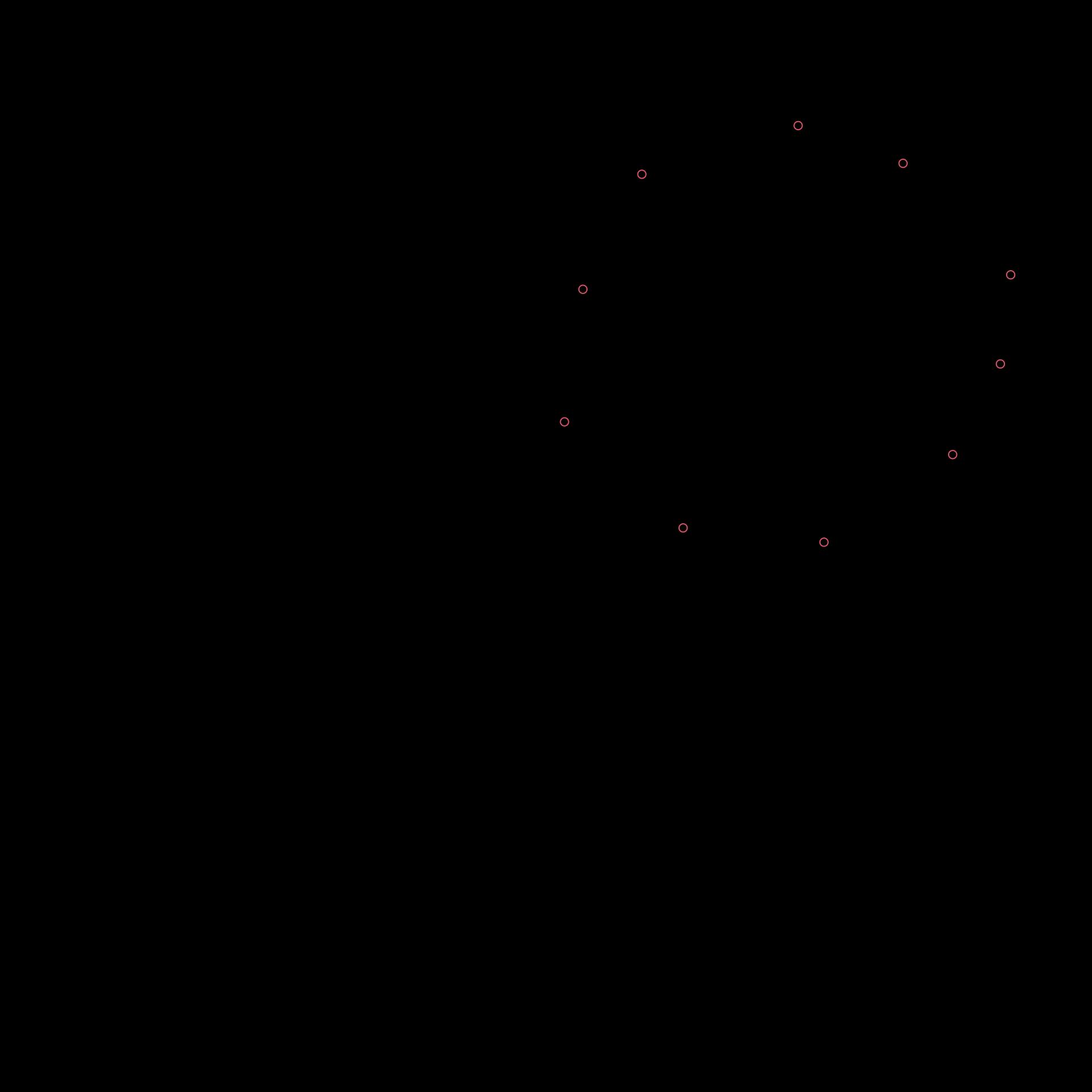

plot(
  denoised$X, 
  denoised$Y,
  col = factor(denoised$person)
)

Filtered and binned positions as achieved through the denoiser function.

Note that to make sense of the time variable, one should realize that for any $i \in \{0, 1, \cdots T\}$, we define the bins as $(t_i, t_i + \Delta t]$ except for the first bin, which is defined as $[t_i, t_i + \Delta t]$.